Summarizing conscious experience

There’s a puzzle for implementation of probabilistic reasoning in human beings. This is that the start of the reasoning process in humans is conscious experience, and it’s not totally clear how we should update on conscious experiences.

Jeffreys defined a summary of an experience E as a set B of propositions {B1, B2, … Bn} such that for all other propositions in your belief system A, P(A | B) = P(A | B, E).

In other words, B is a minimal set of propositions that fully screens off your experience.

This is a useful concept because summary sentences allow you to isolate everything that is epistemically relevant about conscious experience. if you have a summary B of an experience E, then you only need to know P(A | B) and P(B | E) in order to calculate P(A | E).

Notice that the summary set is subjective; it is defined only in terms of properties of your personal belief network. The set of facts that screens off E for you might be different from the set of facts that screens it off for somebody else.

Quick example.

Consider a brief impression by candlelight of a cloth held some distance away from you. Call this experience E.

Suppose that all you could decipher from E is that the cloth was around 2 meters away from you, and that it was either blue (with probability 60%) or green (with probability 40%). Then the summary set for E might be {“The cloth is blue”, “The cloth is green”, “The cloth is 2 meters away from you”, “The cloth is 3 meters away from you”, etc.}.

If this is the right summary set, then the probabilities P(“The cloth is blue”), P(“The cloth is green”) and P(“The cloth is x meters away from you”) should screen off E from the rest of your beliefs.

One trouble is that it’s not exactly obvious how to go about converting a given experience into a set of summary propositions. We could always be leaving something out. For instance, one more thing we learned upon observing E was the proposition “I can see light.” This is certainly not screened off by the other propositions so far, so we need to add it in as well.

But how do we know that we’ve gotten everything now? If we think a little more, we realize that we have also learned something about the nature of the light given off by the candle flame. We learn that it is capable of reflecting the color of light that we saw!

But now this additional consideration is related to how we interpret the color of the cloth. In other words, not only might we be missing something from our summary set, but that missing piece might be relevant to how we interpret the others.

I’d like to think more about this question: In general, how do we determine the set of propositions that screens off a given experience from the rest of your beliefs? Ultimately, to be able to coherently assess the impact of experiences on your web of beliefs, your model of reality must contain a model of yourself as an experiencer.

The nature of this model is pretty interesting from a philosophical perspective. Does it arise organically out of factual beliefs about the physical world? Well, this is what a physicalist would say. To me, it seems quite plausible that modeling yourself as a conscious experiencer would require a separate set of rules relating physical happenings to conscious experiences. How we should model this set of rules as a set of a priori hypotheses to be updated on seems very unclear to me.

Simple induction

In front of you is a coin. You don’t know the bias of this coin, but you have some prior probability distribution over possible biases (between 0: always tails, and 1: always heads). This distribution has some statistical properties that characterize it, such as a standard deviation and a mean. And from this prior distribution, you can predict the outcome of the next coin toss.

Now the coin is flipped and lands heads. What is your prediction for the outcome of the next toss?

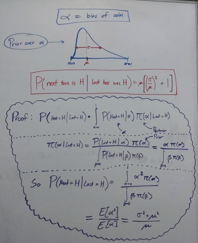
This is a dead simple example of a case where there is a correct answer to how to reason inductively. It is as correct as any deductive proof, and derives a precise and unambiguous result:

Fixed

This is a law of rational thought, just as rules of logic are laws of rational thought. It’s interesting to me how the understanding of the structure of inductive reasoning begins to erode the apparent boundary between purely logical a priori reasoning and supposedly a posteriori inductive reasoning.

Anyway, here’s one simple conclusion that we can draw from the above image: After the coin lands heads, it should be more likely that the coin will land heads next time. After all, the initial credence was µ, and the final credence is µ multiplied by a value that is necessarily greater than 1.

You probably didn’t need to see an equation to guess that for each toss that lands H, future tosses landing H become more likely. But it’s nice to see the fundamental justification behind this intuition.

We can also examine some special cases. For instance, consider a uniform prior distribution (corresponding to maximum initial uncertainty about the coin bias). For this distribution (π = 1), µ = 1/2 and σ = 1/3. Thus, we arrive at the conclusion that after getting one heads, your credence in the next toss landing heads should be 13/18 (72%, up from 50%).

We can get a sense of the insufficiency of point estimates using this example. Two prior distributions with the same average value will respond very differently to evidence, and thus the final point estimate of the chance of H will differ. But what is interesting is that while the mean is insufficient, just the mean and standard deviation suffice for inferring the value of the next point estimate.

In general, the dynamics are controlled by the term σ/µ. As σ/µ goes to zero (which corresponds to a tiny standard deviation, or a very confident prior), our update goes to zero as well. And as σ/µ gets large (either by a weak prior or a low initial credence in the coin being H-biased), the observation of H causes a greater update.

How large can this term possibly get? Obviously, the updated point estimate should asymptote towards 1, but this is not obvious from the form of the equation we have (it looks like σ/µ can get arbitrarily large, forcing our final point estimate to infinity). What we need to do is optimize the updated point estimate, while taking into account the constraints implied by the relationship between σ and µ.

Patterns of inductive inference

I’m currently reading through Judea Pearl’s wonderful book Probabilistic Inference in Intelligent Systems. It’s chock-full of valuable insights into the subtle patterns involved in inductive reasoning.

Here are some of the patterns of reasoning described in Chapter 1, ordered in terms of increasing unintuitiveness. Any good system of inductive inference should be able to accommodate all of the following.

Abduction:

If A implies B, then finding that B is true makes A more likely.

Example: If fire implies smoke, smoke suggests fire.

Asymmetry of inference:

There are two types of inference that function differently: predictive vs explanatory. Predictive inference reasons from causes to consequences, whereas explanatory inference reasons from consequences to causes.

Example: Seeing fire suggests that there is smoke (predictive). Seeing smoke suggests that there is a fire (diagnostic).

Induced Dependency:

If you know A, then learning B can suggest C where it wouldn’t have if you hadn’t known A.

Example: Ordinarily, burglaries and earthquakes are unrelated. But if you know that your alarm is going off, then whether or not there was an earthquake is relevant to whether or not there was a burglary.

Correlated Evidence:

Upon discovering that multiple sources of evidences have a common origin, the credibility of the hypothesis should be decreased.

Example: You learn on a radio report, TV report, and newspaper report that thousands died. You then learn that all three reports got their information from the same source. This decreases the credibility that thousands died.

Explaining away:

Finding a second explanation for an item of data makes the first explanation less credible. If A and B both suggest C, and C is true, then finding that B is true makes A less credible.

Example: Finding that my light bulb emits red light makes it less credible that the red-hued object in my hand is truly red.

Rule of the hypothetical middle:

If two diametrically opposed assumptions impart two different degrees of belief onto a proposition Q, then the unconditional degree of belief should be somewhere between the two.

Example: The plausibility of an animal being able to fly is somewhere between the plausibility of a bird flying and the plausibility of a non-bird flying.

Defeaters or Suppressors:

Even if as a general rule B is more likely given A, this does not necessarily mean that learning A makes B more credible. There may be other elements in your knowledge base K that explain A away. In fact, learning B might cause A to become less likely (Simpson’s paradox). In other words, updating beliefs must involve searching your entire knowledge base for defeaters of general rules that are not directly inferentially connected to the evidence you receive.

Example 1: Learning that the ground is wet does not permit us to increase the certainty of “It rained”, because the knowledge base might contain “The sprinkler is on.”
Example 2: You have kidney stones and are seeking treatment. You additionally know that Treatment A makes you more likely to recover from kidney stones than Treatment B. But if you also have the background information that your kidney stones are large, then your recovery under Treatment A becomes less credible than under Treatment B.

Non-Transitivity:

Even if A suggests B and B suggests C, this does not necessarily mean that A suggests C.

Example 1: Your card being an ace suggests it is an ace of clubs. If your card is an ace of clubs, then it is a club. But if it is an ace, this does not suggest that it is a club.
Example 2: If the sprinkler was on, then the ground is wet. If the ground is wet, then it rained. But it’s not the case that if the sprinkler was on, then it rained.

Non-detachment:

Just learning that a proposition has changed in credibility is not enough to analyze the effects of the change; the reason for the change in credibility is relevant.

Example: You get a phone call telling you that your alarm is going off. Worried about a burglar, you head towards your home. On the way, you hear a radio announcement of an earthquake near your home. This makes it more credible that your alarm really is going off, but less credible that there was a burglary. In other words, your alarm going off decreased the credibility of a burglary, because it happened as a result of the earthquake, whereas typically an alarm going off would make a burglary more credible.

✯✯✯

All of these patterns should make a lot of sense to you when you give them a bit of thought. It turns out, though, that accommodating them in a system of inference is no easy matter.

Pearl distinguishes between extensional and intensional systems, and talks about the challenges for each approach. Extensional systems (including fuzzy logic and non-monotonic logic) focus on extending the truth values of propositions from {0,1} to a continuous range of uncertainty [0, 1], and then modifying the rules according to which propositions combine (for instance, the proposition “A & B” has the truth value min{A, B} in some extensional systems and A*B in others). The locality and simplicity of these combination rules turns out to be their primary failing; they lack the subtlety and nuance required to capture the complicated reasoning patterns above. Their syntactic simplicity makes them easy to work with, but curses them with semantic sloppiness.

On the other hand, intensional systems (like probability theory) involve assigning a function from entire world-states (rather than individual propositions) to degrees of plausibility. This allows for the nuance required to capture all of the above patterns, but results in a huge blow up in complexity. True perfect Bayesianism is ridiculously computationally infeasible, as the operation of belief updating blows up exponentially as the number of atomic propositions increases. Thus, intensional systems are semantically clear, but syntactically messy.

A good summary of this from Pearl (p 12):

We have seen that handling uncertainties is a rather tricky enterprise. It requires a fine balance between our desire to use the computational permissiveness of extensional systems and our ability to refrain from committing semantic sins. It is like crossing a minefield on a wild horse. You can choose a horse with good instincts, attach certainty weights to it and hope it will keep you out of trouble, but the danger is real, and highly skilled knowledge engineers are needed to prevent the fast ride from becoming a disaster. The other extreme is to work your way by foot with a semantically safe intensional system, such as probability theory, but then you can hardly move, since every step seems to require that you examine the entire field afresh.

The challenge for extensional systems is to accommodate the nuance of correct inductive reasoning.

The challenge for intensional systems is to maintain their semantic clarity while becoming computationally feasible.

Pearl solves the second challenge by supplementing Bayesian probability theory with causal networks that give information about the relevance of propositions to each other, drastically simplifying the tasks of inference and belief propagation.

One more insight from Chapter 1 of the book… Pearl describes four primitive qualitative relationships in everyday reasoning: likelihood, conditioning, relevance, and causation. I’ll give an example of each, and how they are symbolized in Pearl’s formulation.

1. Likelihood (“Tim is more likely to fly than to walk.”)
P(A)

2. Conditioning (“If Tim is sick, he can’t fly.”)
P(A | B)

3. Relevance (“Whether Tim flies depends on whether he is sick.”)
A B

4. Causation (“Being sick caused Tim’s inability to fly.”)
P(A | do B)

The challenge is to find a formalism that fits all four of these, while remaining computationally feasible.

Variational Bayesian inference

Today I learned a cool trick for practical implementation of Bayesian inference.

Bayesians are interested in calculating posterior probability distributions of unobserved parameters X, given data (which consists of the values of observed parameters Y).

To do so, they need only know the form of the likelihood function (the probability of Y given X) and their own prior distribution over X. Then they can apply Bayes’ rule…

P(X | Y) = P(Y | X) P(X) / P(Y)

… and voila, Bayesian inference complete.

The trickiest part of this process is calculating the term in the denominator, the marginal likelihood P(Y). Trying to calculate this term analytically is typically  very computationally expensive – it involves a sum over all possible values of the parameters of the likelihood multiplied by the prior. If Y is drawn from a continuous infinity of possible parameter values, then calculating the marginal likelihood amounts to solving a (typically completely intractable) integral.

P(Y) = ∫ P(Y | X) P(X) dX

Variational Bayesian inference is a procedure that solves this problem through a clever trick.

We start by searching for a posterior in a space of functions F that are easily integrable.

Our goal is not to find the exact form of the posterior, although if we do, that’s great. Instead, we want to find the function Q(X) within F that is as close to the posterior P(X | Y) as possible.

Distance between probability distributions is typically calculated by the information divergence D(Q, P), which is defined by…

D(Q, P) = ∫ Q(X) log(Q(X) / P(X|Y)) dX

To explicitly calculate and minimize this, we would need to know the form of the posterior P(X | Y) from the start. But let’s plug in the definition of conditional probability…

P(X | Y) = P(X, Y) / P(Y)

D(Q, P) = ∫ Q(X) log(Q(X) P(Y) / P(X, Y)) dX
= ∫ Q(X) log(Q(X) / P(X, Y)) dX  +  ∫ Q(X) log P(Y) dX

The second term is easily calculated. Since log(P(Y)) is not a function of X, the integral just becomes…

∫ Q(X) log P(Y) dX = log P(Y)

Rearranging, we get…

log P(Y) = D(Q, P)  –  ∫ Q(X) log(Q(X) / P(X, Y)) dX

The second term depends on Q(X) and the joint probability P(X, Y), which we can calculate easily as the product of the likelihood P(Y | X) and the prior P(X). We name it the variational free energy, L(Q).

log P(Y) = D(Q, P) + L(Q)

Now, on the left-hand side we have the log of the marginal likelihood, and on the right we have the information distance plus the variational free energy.

Notice that the left side is not a function of Q. This is really important! It tells us that if we’re trying to vary Q to minimize D(Q, P), then the right side will be a constant quantity.

In other words, any increase in L(Q) is necessarily a decrease in D(Q, P). What this means is that the Q that minimizes D(Q, P) is the same thing as the Q that maximizes L(Q)!

We can use this to minimize D(Q, P) without ever explicitly knowing P.

Recalling the definition of the variational free energy, we have…

L(Q) = – ∫ Q(X) log(Q(X) / P(X, Y)) dX
= ∫ Q(X) log P(X, Y) dX – ∫ Q(X) log Q(X) dX

Both of these integrals are computable insofar as we made a good choice for the function space F. Thus we can exactly find Q*, the best approximation to P in F. Then, knowing Q*, we can calculate L(Q*), which serves as a lower bound on the log of the marginal likelihood P(Y).

log P(Y) = D(Q, P) + L(Q)
so log P(Y) ≥ L(Q*)

Summing up…

  1. Variational Bayesian inference approximates the posterior probability P(X | Y) with a function Q(X) in the function space F.
  2. We find the function Q* that is as similar as possible to P(X | Y) by maximizing L(Q).
  3. L(Q*) gives us a lower bound on the log of the marginal likelihood, log P(Y).

Objective Bayesianism and choices of concepts

Bayesians believe in treating belief probabilistically, and updating credences via Bayes’ rule. They face the problem of how to set priors – while probability theory gives a clear prescription for how to update beliefs, it doesn’t tell you what credences you should start with before getting any evidence.

Bayesians are thus split into two camps: objective Bayesians and subjective Bayesians. Subjective Bayesians think that there are no objectively correct priors. A corollary to this is that there are no correct answers to what somebody should believe, given their evidence.

Objective Bayesians disagree. Different variants specify different procedures for determining priors. For instance, the principle of indifference (POI) prescribes that the proper priors are those that are indifferent between all possibilities. If you have N possibilities, then according to the POI, you should distribute your priors credences evenly (1/N each). If you are considering a continuum of hypotheses (say, about the mass of an object), then the principle of indifference says that your probability density function should be uniform over all possible masses.

Now, here’s a problem for objective Bayesians.

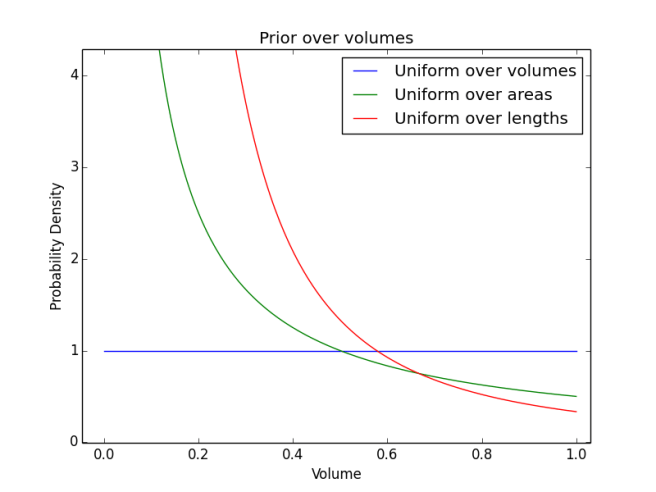
You are going to be handed a cube, and all that you know about it is that it is smaller than 1 cm3. What should your prior distribution over possible cubes you might be handed look like?

Naively applying the POI, you might evenly distribute your credences across all volumes from 0 cm3 to 1 cm3 (so that there is a 50% chance that the cube has a volume less than .50 cm3 and a 50% chance its volume is between greater than .50 cm3).

But instead of choosing to be indifferent over possible volumes, we could equally well have chosen to be indifferent over possible side areas, or side lengths. The key point is that these are all different distributions. If we spread our credences evenly across possible side lengths from 0 cm to 1 cm, then we would have a distribution with a 50% chance that the cube has a volume less than .125 cm3 and a 50% chance that the volume is greater than this.

Cube puzzle

In other words, our choice of concepts (edge length vs side area vs volume) ends up determining the shape of our prior. Insofar as there is no objectively correct choice of concepts to be using, there is no objectively correct prior distribution.

I’ve known about this thought experiment for a while, but only recently internalized how serious of a problem it presents. It essentially says that your choice of priors is hostage to your choice of concepts, which is a pretty unsavory idea. In some cases, which concept to choose is very non-obvious (e.g. length vs area vs volume). In others, there are strong intuitions about some concepts being better than others.

The most famous example of this is contained in Nelson Goodman’s “new riddle of induction.” He proposes a new concept grue, which is defined as the set of objects that are either observed before 2100 and green, or observed after 2100 and blue. So if you spot an emerald before 2100, it is grue. So is a blue ball that you spot after 2100. But if you see an emerald after 2100, it will not be grue.

To characterize objects like this emerald that is observed after 2100, Goodman also creates another concept bleen, which is the inverse of grue. The set of bleen objects is composed of blue objects observed before 2100 and green objects observed after 2100.

Now, if we run ordinary induction using the concepts grue and bleen, we end up making bizarre predictions. For instance, say we observe many emeralds before 2100, and always found them to be green. By induction, we should infer that the next emerald we observe after 2100 is very likely going to be green as well. But if we thought in terms of the concepts grue and bleen, then we would say that all our observations of emeralds so far have provided inductive support for the claim “All emeralds are grue.” The implication of this is that the emeralds we observe after time 2100 will very likely also be grue (and thus blue).

In other words, by simply choosing a different set of fundamental concepts to work with, we end up getting an entirely different prediction about the future.

Here’s one response that you’ve probably already thought of: “But grue and bleen are such weird artificial choices of concepts! Surely we can prefer green/blue over bleen/grue on the basis of the additional complexity required in specifying the transition time 2100?”

The problem with this is that we could equally well define green and blue in terms of grue and bleen:

Green = grue before 2100 or bleen after 2100
Blue = bleen before 2100 or grue after 2100

If for whatever reason somebody had grue and bleen as their primitive concepts, they would see green and blue as the concepts that required the additional complexity of the time specification.

“Okay, sure, but this is only if we pretend that color is something that doesn’t emerge from lower physical levels. If we tried specifying the set of grue objects in terms of properties of atoms, we’d have a lot harder time than if we tried specifying the set of green or blue objects in terms of properties of atoms.”

This is right, and I think it’s a good response to this particular problem. But it doesn’t work as a response to a more generic form of the dilemma. In particular, you can construct a grue/bleen-style set of concepts for whatever you think is the fundamental level of reality. If you think electrons and neutrinos are undecomposable into smaller components, then you can imagine “electrinos” and “neuctrons.” And now we have the same issue as before… thinking in terms of electrinos would lead us to conclude that all electrons will suddenly transform into neutrinos in 2100.

The type of response I want to give is that concepts like “electron” and “neutrino” are preferable to concepts like “electrinos” and “neuctrons” because they mirror the structure of reality. Nature herself computes electrons, not electrinos.

But the problem is that we’re saying that in order to determine which concepts we should use, we need to first understand the broad structure of reality. After which we can run some formal inductive schema to, y’know, figure out the broad structure of reality.

Said differently, we can’t really appeal to “the structure of reality” to determine our choices of concepts, since our choices of concepts end up determining the results of our inductive algorithms, which are what we’re relying on to tell us the structure of reality in the first place!

This seems like a big problem to me, and I don’t know how to solve it.

Regularization as approximately Bayesian inference

In an earlier post, I showed how the procedure of minimizing sum of squares falls out of regular old frequentist inference. This time I’ll do something similar, but with regularization and Bayesian inference.

Regularization is essentially a technique in which you evaluate models in terms of not just their fit to the data, but also the values of the parameters involved. For instance, say you are modeling some data with a second-order polynomial.

M = { f(x) = a + bx + cx2 | a, b, c ∈ R }
D = { (x1, y1), …, (xN, yN) }

We can evaluate our model’s fit to the data with SOS:

SOS = ∑ (yn – f(xn))2

Minimizing SOS gives us the frequentist answer – the answer that best fits the data. But what if we suspect that the values of a, b, and c are probably small? In other words, what if we have an informative prior about the parameter values? Then we can explicitly add on a penalty term that increases the SOS, such as…

SOS with L1 regularization = k1 |a| + k2 |b| + k3 |c| + ∑ (yn – f(xn))2

The constants k1, k2, and k3 determine how much we will penalize each parameter a, b, and c. This is not the only form of regularization we could use, we could also use the L2 norm:

SOS with L2 regularization = k1 a2 + k2 b2 + k3 c2 + ∑ (yn – f(xn))2

In both of these cases, the regularized SOS term grows as the values of the parameters grow. This makes the optimal choice of curve take into account not only the fit to data, but the desired size of the parameters.

You might, having heard of this procedure, already suspect it of having a Bayesian bent. The notion of penalizing large parameter values on the basis of a prior suspicion that the values should be small sounds a lot like what the Bayesian would call “low priors on high parameter values.”

We’ll now make the connection explicit.

Frequentist inference tries to select the theory that makes the data most likely. Bayesian inference tries to select the theory that is made most likely by the data. I.e. frequentists choose f to maximize P(D | f), and Bayesians choose f to maximize P(f | D).

Assessing P(f | D) requires us to have a prior over our set of functions f, which we’ll call π(f).

P(f | D) = P(D | f) π(f) / P(D)

We take a logarithm to make everything easier:

log P(f | D) = log P(D | f) + log π(f) – log P(D)

We already evaluated P(D | f) in the last post, so we’ll just plug it in right away.

log P(f | D) = – SOS/2σ2 – N/2 log(2πσ2)) + log π(f) – log P(D)

Since we are maximizing with respect to f, two of these terms will fall away.

log P(f | D) = – SOS/2σ2 + log π(f) + constant

Now we just have to decide on the form of π(f). Since the functional form of f is determined by the values of the parameters {a, b, c}, π(f) = π(a, b, c). One plausible choice is a Gaussian centered around the values of each parameter:

π(f) = exp( -a2 / 2σa2 ) exp( -b2 / 2σb2 ) exp( -c2 / 2σc2 ) / √(8π3σa2σb2σc2)
log π(f) = -a2/2σa2 – b2/2σb2 – c2/2σc2 – ½ log(8π3σa2σb2σc2)

Now, throwing out terms that don’t depend on the values of the parameters, we find:

log P(f | D) = – SOS/2σ2 -a2/2σa2 – b2/2σb2 – c2/2σc2 + constant

This is exactly L2 regularization, where each kn = σ2n2. In other words, L2 regularization is Bayesian inference with Gaussian priors over the parameters!

What priors does L1 regularization correspond to?

log π(f) = -k1 |a| – k2 |b| – k3 |c|
π(a, b, c) = e-k1|a| e-k2|b| e-k3|a|

I.e. the L1 regularization prior is an exponential distribution.

This can be easily extended to any regularization technique. This is a way to get some insight into what your favorite regularization methods mean. They are ultimately to be cashed out in the form of your prior knowledge of the parameters!

Why minimizing sum of squares is equivalent to frequentist inference

(This will be the first in a short series of posts describing how various commonly used statistical methods are approximate versions of frequentist, Bayesian, and Akaike-ian inference)

Suppose that we have some data D = { (x₁, y₁), (x₂, y₂), … , (xɴ, yɴ) }, and a candidate function y = f(x).

Frequentist inference involves the assessment of the likelihood of the data given this candidate function: P(D | f).

Since D is composed of N independent data points, we can assess the probability of each data point separately, and multiply them all together.

P(D | f) = P(x₁, y₁ | f) P(x₂, y₂ | f) … P(xɴ, yɴ | f)

So now we just need to answer the question: What is P(x, y | f)?

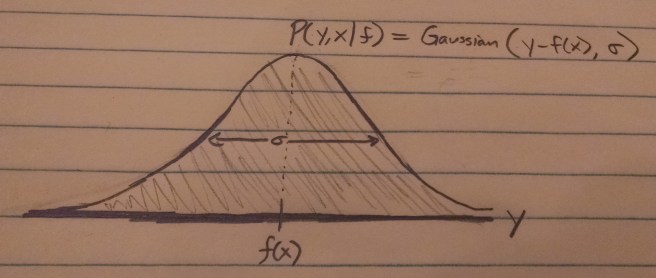
f predicts that for the value x, the most likely y-value is f(x).

The other possible y-values will be normally distributed around f(x).

IMG_20180522_192208774

The equation for this distribution is a Gaussian:

P(x, y | f) = exp[ -(y – f(x))² / 2σ² ] / √(2πσ²)

Now that we know how to find P(x, y | f), we can easily calculate P(D | F)!

P(D | f) = exp[ -(y – f(x))² / 2σ² ] /√(2πσ²) ・ exp[ -(y – f(x))² / 2σ² ] / √(2πσ²) … exp[ -(y – f(x))² / 2σ² ] / √(2πσ²)
= exp[ -(y – f(x))² / 2σ² ] ・ exp[ -(y – f(x))² / 2σ² ] … exp[ -(y – f(x))² / 2σ² ] / (2πσ²)N/2

Products are messy and logarithms are monotonic, so log(P(D | f)) is easier to work with: it turns the product into a sum.

log P(D | f) = log( exp[ -(y₁ – f(x₁))² / 2σ² ] … exp[ -(yɴ – f(xɴ))² / 2σ² ] / (2πσ²)N/2 )
= log( exp[ -(y₁ – f(x₁))² / 2σ² ] ) + … log( exp[ -(yɴ – f(xɴ))² / 2σ² ] ) – N/2 log(2πσ²)
= -(y₁ – f(x₁))² / 2σ² ) + -(yɴ – f(xɴ))² / 2σ² ) – N/2 log(2πσ²)
= -1/2σ² [ (y₁ – f(x₁))² + … +(yɴ – f(xɴ))² ] – N/2 log(2πσ²)

Now notice that the sum of squares just naturally pops out!

SOS = (y₁ – f(x₁))² + … + (yɴ – f(xɴ))²
log P(D | f) = -SOS/2σ² – N/2 log(2πσ²)

Frequentist inference chooses f to maximize P(D | f). We can now immediately see why this is equivalent to minimizing SOS!

argmax{ P(D | f) }
= argmax{ log P(D | f) }
= argmax{ – SOS/2σ² – N/2 log(2πσ²) }
= argmin{ SOS/2σ² + N/2 log(2πσ²) }
= argmin{ SOS/2σ² }
= argmin{ SOS }

Next, we’ll go Bayesian…

Short and sweet proof of the f(xy) = f(x) + f(y) logarithmic property

If you want a continuously differentiable function f(x) from the reals to the reals that has the property that for all real x and y, f(xy) = f(x) + f(y), then this function must take the form f(x) = k log(x) for some real k.

A proof of this just popped into my head in the shower. (As always with shower-proofs, it was slightly wrong, but I worked it out and got it right after coming out).

I haven’t seen it anywhere before, and it’s a lot simpler than previous proofs that I’ve encountered.

Here goes:

f(xy) = f(x) + f(y)

differentiate w.r.t. x…
f'(xy) y = f'(x)

differentiate w.r.t. y…
f”(xy) xy + f'(xy) = 0

rearrange, and rename xy to z…
f”(z) = -f'(z)/z

solve for f'(z) with standard 1st order DE techniques…
df’/f’ = – dz/z
log(f’) = -log(z) + constant
f’ = constant/z

integrate to get f…
f(z) = k log(z) for some constant k

And that’s the whole proof!

As for why this is interesting to me… the equation f(xy) = f(x) + f(y) is very easy to arrive at in constructing functions with desirable features. In words, it means that you want the function’s outputs to be additive when the inputs are multiplicative.

One example of this, which I’ve written about before, is formally quantifying our intuitive notion of surprise. We formalize surprise by asking the question: How surprised should you be if you observe an event that you thought had a probability P? In other words, we treat surprise as a function that takes in a probability and returns a scalar value.

We can lay down a few intuitive desideratum for our formalization of surprise, and one such desideratum is that for independent events E and F, our surprise at them both happening should just be the sum of the surprise at each one individually. In other words, we want surprise to be additive for independent events E and F.

But if E and F are independent, then the joint probability P(E, F) is just the product of the individual probabilities: P(E, F) = P(E) P(F). In other words, we want our outputs to be additive, when our inputs are multiplicative!

This automatically gives us that the form of our surprise function must be k log(z). To spell it out explicitly…

Desideratum: Surprise(P(E, F)) = Surprise(P(E)) + Surprise(P(F))

But P(E,F) = P(E) P(F), so…
Surprise(P(E) P(F)) = Surprise(P(E)) + Surprise(P(F))

Renaming P(E) to x and P(F) to y…
Surprise(xy) = Surprise(x) + Surprise(y)

Thus, by the above proof…
Surprise(x) = k log(x) for some constant k

That’s a pretty strong constraint for some fairly weak inputs!

That’s basically why I find this interesting: it’s a strong constraint that comes out of an intuitively weak condition.

Galileo and the Schelling point improbability principle

An alternative history interaction between Galileo and his famous statistician friend

***

In the year 1609, when Galileo Galilei finished the construction of his majestic artificial eye, the first place he turned his gaze was the glowing crescent moon. He reveled in the crevices and mountains he saw, knowing that he was the first man alive to see such a sight, and his mind expanded as he saw the folly of the science of his day and wondered what else we might be wrong about.

For days he was glued to his telescope, gazing at the Heavens. He saw the planets become colorful expressive spheres and reveal tiny orbiting companions, and observed the distant supernova which Kepler had seen blinking into existence only five years prior. He discovered that Venus had phases like the Moon, that some apparently single stars revealed themselves to be binaries when magnified, and that there were dense star clusters scattered through the sky. All this he recorded in frantic enthusiastic writing, putting out sentences filled with novel discoveries nearly every time he turned his telescope in a new direction. The universe had opened itself up to him, revealing all its secrets to be uncovered by his ravenous intellect.

It took him two weeks to pull himself away from his study room for long enough to notify his friend Bertolfo Eamadin of his breakthrough. Eamadin was a renowned scholar, having pioneered at age 15 his mathematical theory of uncertainty and created the science of probability. Galileo often sought him out to discuss puzzles of chance and randomness, and this time was no exception. He had noticed a remarkable confluence of three stars that were in perfect alignment, and needed the counsel of his friend to sort out his thoughts.

Eamadin arrived at the home of Galileo half-dressed and disheveled, obviously having leapt from his bed and rushed over immediately upon receiving Galileo’s correspondence. He practically shoved Galileo out from his viewing seat and took his place, eyes glued with fascination on the sky.

Galileo allowed his friend to observe unmolested for a half-hour, listening with growing impatience to the ‘oohs’ and ‘aahs’ being emitted as the telescope swung wildly from one part of the sky to another. Finally, he interrupted.

Galileo: “Look, friend, at the pattern I have called you here to discuss.”

Galileo swiveled the telescope carefully to the position he had marked out earlier.

Eamadin: “Yes, I see it, just as you said. The three stars form a seemingly perfect line, each of the two outer ones equidistant from the central star.”

Galileo: “Now tell me, Eamadin, what are the chances of observing such a coincidence? One in a million? A billion?”

Eamadin frowned and shook his head. “It’s certainly a beautiful pattern, Galileo, but I don’t see what good a statistician like myself can do for you. What is there to be explained? With so many stars in the sky, of course you would chance upon some patterns that look pretty.”

Galileo: “Perhaps it seems only an attractive configuration of stars spewed randomly across the sky. I thought the same myself. But the symmetry seemed too perfect. I decided to carefully measure the central angle, as well as the angular distance distended by the paths from each outer star to the central one. Look.”

Galileo pulled out a sheet of paper that had been densely scribbled upon. “My calculations revealed the central angle to be precisely 180.000º, with an error of ± .003º. And similarly, I found the difference in the two angular distances to be .000º, with a margin of error of ± .002º.”

Eamadin: “Let me look at your notes.”

Galileo handed over the sheets to Eamadin. “I checked over my calculations a dozen times before writing you. I found the angular distances by approaching and retreating from this thin paper, which I placed between the three stars and me. I found the distance at which the thin paper just happened to cover both stars on one extreme simultaneously, and did the same for the two stars on the other extreme. The distance was precisely the same, leaving measurement error only for the thickness of the paper, my distance from it, and the resolution of my vision.”

Eamadin: “I see, I see. Yes, what you have found is a startlingly clear pattern. A similarity in distance and precision of angle this precise is quite unlikely to be the result of any natural phenomenon… ”

Galileo: “Exactly what I thought at first! But then I thought about the vast quantity of stars in the sky, and the vast number of ways of arranging them into groups of three, and wondered if perhaps in fact such coincidences might be expected. I tried to apply your method of uncertainty to the problem, and came to the conclusion that the chance of such a pattern having occurred through random chance is one in a thousand million! I must confess, however, that at several points in the calculation I found myself confronted with doubt about how to progress and wished for your counsel.”

Eamadin stared at Galileo’s notes, then pulled out a pad of his own and began scribbling intensely. Eventually, he spoke. “Yes, your calculations are correct. The chance of such a pattern having occurred to within the degree of measurement error you have specified by random forces is 10-9.”

Galileo: “Aha! Remarkable. So what does this mean? What strange forces have conspired to place the stars in such a pattern? And, most significantly, why?”

Eamadin: “Hold it there, Galileo. It is not reasonable to jump from the knowledge that the chance of an event is remarkably small to the conclusion that it demands a novel explanation.”

Galileo: “How so?”

Eamadin: “I’ll show you by means of a thought experiment. Suppose that we found that instead of the angle being 180.000º with an experimental error of .003º, it was 180.001º with the same error. The probability of this outcome would be the same as the outcome we found – one in a thousand million.”

Galileo: “That can’t be right. Surely it’s less likely to find a perfectly straight line than a merely nearly perfectly straight line.”

Eamadin: “While that is true, it is also true that the exact calculation you did for 180.000º ± .003º would apply for 180.001º ± .003º. And indeed, it is less likely to find the stars at this precise angle, than it is to find the stars merely near this angle. We must compare like with like, and when we do so we find that 180.000º is no more likely than any other angle!”

Galileo: “I see your reasoning, Eamadin, but you are missing something of importance. Surely there is something objectively more significant about finding an exactly straight line than about a nearly straight line, even if they have the same probability. Not all equiprobable events should be considered to be equally important. Think, for instance, of a sequence of twenty coin tosses. While it’s true that the outcome HHTHTTTTHTHHHTHHHTTH has the same probability as the outcome HHHHHHHHHHHHHHHHHHHH, the second is clearly more remarkable than the first.”

Eamadin: “But what is significance if disentangled from probability? I insist that the concept of significance only makes sense in the context of my theory of uncertainty. Significant results are those that either have a low probability or have a low conditional probability given a set of plausible hypotheses. It is this second class that we may utilize in analyzing your coin tossing example, Galileo. The two strings of tosses you mention are only significant to different degrees in that the second more naturally lends itself to a set of hypotheses in which the coin is heavily biased towards heads. In judging the second to be a more significant result than the first, you are really just saying that you use a natural hypothesis class in which probability judgments are only dependent on the ratios of heads and tails, not the particular sequence of heads and tails. Now, my question for you is: since 180.000º is just as likely as 180.001º, what set of hypotheses are you considering in which the first is much less likely than the second?”

Galileo: “I must confess, I have difficulty answering your question. For while there is a simple sense in which the number of heads and tails is a product of a coin’s bias, it is less clear what would be the analogous ‘bias’ in angles and distances between stars that should make straight lines and equal distances less likely than any others. I must say, Eamadin, that in calling you here, I find myself even more confused than when I began!”

Eamadin: “I apologize, my friend. But now let me attempt to disentangle this mess and provide a guiding light towards a solution to your problem.”

Galileo: “Please.”

Eamadin: “Perhaps we may find some objective sense in which a straight line or the equality of two quantities is a simpler mathematical pattern than a nearly straight line or two nearly equal quantities. But even if so, this will only be a help to us insofar as we have a presumption in favor of less simple patterns inhering in Nature.”

Galileo: “This is no help at all! For surely the principle of Ockham should push us towards favoring more simple patterns.”

Eamadin: “Precisely. So if we are not to look for an objective basis for the improbability of simple and elegant patterns, then we must look towards the subjective. Here we may find our answer. Suppose I were to scribble down on a sheet of paper a series of symbols and shapes, hidden from your view. Now imagine that I hand the images to you, and you go off to some unexplored land. You explore the region and draw up cartographic depictions of the land, having never seen my images. It would be quite a remarkable surprise were you to find upon looking at my images that they precisely matched your maps of the land.”

Galileo: “Indeed it would be. It would also quickly lend itself to a number of possible explanations. Firstly, it may be that you were previously aware of the layout of the land, and drew your pictures intentionally to capture the layout of the land – that is, that the layout directly caused the resemblance in your depictions. Secondly, it could be that there was a common cause between the resemblance and the layout; perhaps, for instance, the patterns that most naturally come to the mind are those that resemble common geographic features. And thirdly, included only for completion, it could be that your images somehow caused the land to have the geographic features that it did.”

Eamadin: “Exactly! You catch on quickly. Now, this case of the curious coincidence of depiction and reality is exactly analogous to your problem of the straight line in the sky. The straight lines and equal distances are just like patterns on the slips of paper I handed to you. For whatever reason, we come pre-loaded with a set of sensitivities to certain visual patterns. And what’s remarkable about your observation of the three stars is that a feature of the natural world happens to precisely align with these patterns, where we would expect no such coincidence to occur!”

Galileo: “Yes, yes, I see. You are saying that the improbability doesn’t come from any objective unusual-ness of straight lines or equal distances. Instead, the improbability comes from the fact that the patterns in reality just happen to be the same as the patterns in my head!”

Eamadin: “Precisely. Now we can break down the suitable explanations, just as you did with my cartographic example. The first explanation is that the patterns in your mind were caused by the patterns in the sky. That is, for some reason the fact that these stars were aligned in this particular way caused you to by psychologically sensitive to straight lines and equal quantities.”

Galileo: “We may discard this explanation immediately, for such sensitivities are too universal and primitive to be the result of a configuration of stars that has only just now made itself apparent to me.”

Eamadin: “Agreed. Next we have a common cause explanation. For instance, perhaps our mind is naturally sensitive to visual patterns like straight lines because such patterns tend to commonly arise in Nature. This natural sensitivity is what feels to us on the inside as simplicity. In this case, you would expect it to be more likely for you to observe simple patterns than might be naively thought.”

Galileo: “We must deny this explanation as well, it seems to me. For the resemblance to a straight line goes much further than my visual resolution could even make out. The increased likelihood of observing a straight line could hardly be enough to outweigh our initial naïve calculation of the probability being 10-9. But thinking more about this line of reasoning, it strikes me that you have just provided an explanation the apparent simplicity of the laws of Nature! We have developed to be especially sensitive to patterns that are common in Nature, we interpret such patterns as ‘simple’, and thus it is a tautology that we will observe Nature to be full of simple patterns.”

Eamadin: “Indeed, I have offered just such an explanation. But it is an unsatisfactory explanation, insofar as one is opposed to the notion of simplicity as a purely subjective feature. Most people, myself included, would strongly suggest that a straight line is inherently simpler than a curvy line.”

Galileo: “I feel the same temptation. Of course, justifying a measure of simplicity that does the job we want of it is easier said than done. Now, on to the third explanation: that my sensitivity to straight lines has caused the apparent resemblance to a straight line. There are two interpretations of this. The first is that the stars are not actually in a straight line, and you only think this because of your predisposition towards identifying straight lines. The second is that the stars aligned in a straight line because of these predispositions. I’m sure you agree that both can be reasonably excluded.”

Eamadin: “Indeed. Although it may look like we’ve excluded all possible explanations, notice that we only considered one possible form of the common cause explanation. The other two categories of explanations seem more thoroughly ruled out; your dispositions couldn’t be caused by the star alignment given that you have only just found out about it and the star alignment couldn’t be caused by your dispositions given the physical distance.”

Galileo: “Agreed. Here is another common cause explanation: God, who crafted the patterns we see in Nature, also created humans to have similar mental features to Himself. These mental features include aesthetic preferences for simple patterns. Thus God causes both the salience of the line pattern to humans and the existence of the line pattern in Nature.”

Eamadin: “The problem with this is that it explains too much. Based solely on this argument, we would expect that when looking up at the sky, we should see it entirely populated by simple and aesthetic arrangements of stars. Instead it looks mostly random and scattershot, with a few striking exceptions like those which you have pointed out.”

Galileo: “Your point is well taken. All I can imagine now is that there must be some sort of ethereal force that links some stars together, gradually pushing them so that they end up in nearly straight lines.”

Eamadin: “Perhaps that will be the final answer in the end. Or perhaps we will discover that it is the whim of a capricious Creator with an unusual habit for placing unsolvable mysteries in our paths. I sometimes feel this way myself.”

Galileo: “I confess, I have felt the same at times. Well, Eamadin, although we have failed to find a satisfactory explanation for the moment, I feel much less confused about this matter. I must say, I find this method of reasoning by noticing similarities between features of our mind and features of the world quite intriguing. Have you a name for it?”

Eamadin: “In fact, I just thought of it on the spot! I suppose that it is quite generalizable… We come pre-loaded with a set of very salient and intuitive concepts, be they geometric, temporal, or logical. We should be surprised to find these concepts instantiated in the world, unless we know of some causal connection between the patterns in our mind and the patterns in reality. And by Eamadin’s rule of probability-updating, when we notice these similarities, we should increase our strength of belief in these possible causal connections. In the spirit of anachrony, let us refer to this as the Schelling point improbability principle!”

Galileo: “Sounds good to me! Thank you for your assistance, my friend. And now I must return to my exploration of the Cosmos.”
Why “number of parameters” isn’t good enough

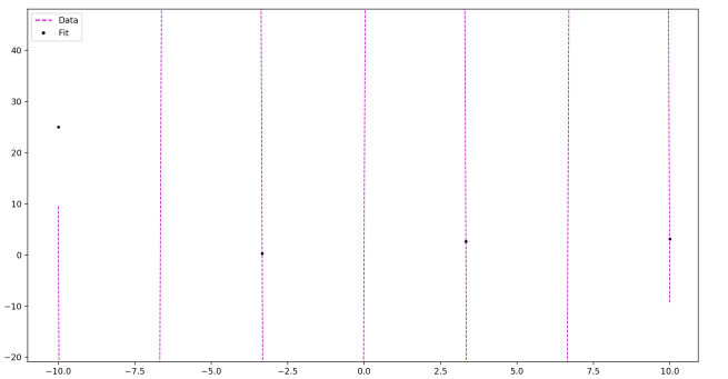
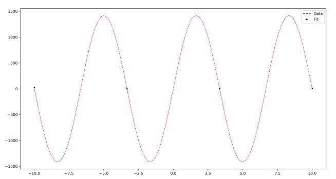
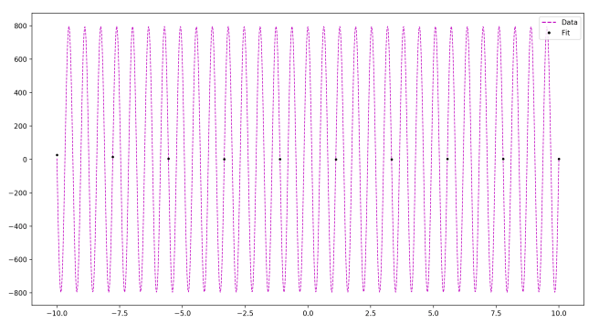
A friend of mine recently pointed out a curious fact. Any set of two-dimensional data whatsoever can be perfectly fit by a simple two-parameter sinusoidal model.

y(x) = A sin(Bx)

Sound wrong? Check it out:

small-sine-zoom.png

Zoomed out:small-sine.png

N = 10 pointssine-overfit.png

As you see, as the number of data points goes up, all you need to do to accommodate this is increase the frequency in your sine function, and adjust the amplitude as necessary. Ultimately, you can fit any data set with a ridiculously quickly oscillating and large-amplitude sine function.

Now, most model selection methods explicitly rely on the parameter count to estimate the potential of a model to overfit. For example, if k is the number of parameters in a model, and L is the log likelihood of the data given the model, we have:

AIC = L – k
BIC = L – k/2・log(N)

This little example represents a fantastic failure of parameter count to successfully do the job AIC and BIC ask of it. Evidently parameter count is too blunt an instrument to do the job we require of it, and we need something with more nuance.

One more example.

For any set of data, if you can perfectly fit a curve to each data point, and if your measurement error σ is an adjustable parameter, then you can take the measurement error to zero to have a fit with infinite accuracy. Now when we evaluate, you find it running off to infinity! Thus our ‘fit to data’ term L goes to infinity, while the model complexity penalty stays a small finite number.

Once again, we see the same lack of nuance dragging us into trouble. The number of parameters might do well at estimating overfitting potential for some types of well-behaved parameters, but it clearly doesn’t do the job universally. What we want is some measure that is sensitive to the potential for some parameters to capture “more” of the space of all possible distributions than others.

And lo and behold, we have such a measure! This is the purpose of information geometry and the volume of a model in the space formed by the Fisher information metric as the penalty for overfitting potential. You can learn more about it in a post I wrote here.