Which paradigm is stronger? When I say logic here, I’ll be referring to standard formal theories like ZFC and Peano arithmetic. If one uses an expansive enough definition to include computability theory, then logic encompasses computation and wins by default.
If you read this post, you might immediately jump to the conclusion that logic is stronger. After all, we concluded that in first order Peano arithmetic one can unambiguously define not only the decidable sets, but the sets decidable with halting oracles, and those decidable with halting oracles for halting oracles, and so on forever. We saw that the Busy Beaver numbers, while undecidable, are definable by a Π1 sentence. And Peano arithmetic is a relatively weak theory; much more is definable in a theory like ZFC!
On the other hand, remember that there’s a difference between what’s absolutely definable and what’s definable-relative-to-ℕ. A set of numbers is absolutely definable if there’s a sentence that is true of just those numbers in every model of PA. It’s definable-relative-to-ℕ if there’s a sentence that’s true of just those numbers in the standard model of PA (the natural numbers, ℕ). Definable-relative-to-ℕ is an unfair standard for the strength of PA, given that PA, and in general no first order system, is able to categorically define the natural numbers. On the other hand, absolute definability is the standard that meets the criterion of “unambiguous definition”. With an absolute definition, there’s no room for confusion about which mathematical structure is being discussed.
All those highly undecidable sets we discussed earlier were only definable-relative-to-ℕ. In terms of what PA is able to define absolutely, it’s limited to only the finite sets. Compare this to what sets of numbers can be decided by a Turing machine. Every finite set is decidable, plus many infinite sets, including the natural numbers!
This is the first example of computers winning out over formal logic in their expressive power. While no first order theory (and in general no theory in a logic with a sound and complete proof system) can categorically define the natural numbers, it’s incredibly simple to write a program that defines that set using the language of PA. In regex, it’s just “S*0”. And here’s a Python script that does the job:
def check(s):
    if s == '':
        return False
    elif s == ‘0’:
        return True
    elif s[0] == ’s’:
        return check(s[1:])
    else:
        return False
We don’t even need a Turing machine for this; we can build a simple finite state machine:
In general, the sets decidable by computer can be much more complicated and interesting than those absolutely definable by a first-order theory. While first-order theories like ZFC have “surrogates” for infinite sets of numbers (ω and its definable subsets), these surrogate sets include nonstandard elements in some models. As a result, ZFC may fail to prove some statements about these sets which hold true of ℕ but fail for nonstandard models. For instance, it may be that the Collatz conjecture is true of the natural numbers but can’t be proven from ZFC. This would be because ZFC’s surrogate for the set of natural numbers (i.e. ω) includes nonstandard elements in some models, and the Collatz conjecture may fail for some such nonstandard elements.
On top of that, by taking just the first Turing jump into uncomputability, computation with a halting oracle, we are able to prove the consistency of ZFC and PA. Since ZFC is recursively axiomatizable, there’s a program that runs forever listing out theorems, such that every theorem is output at some finite point. We can use this to produce a program that looks to see if “0 = 1” is a theorem of ZFC. If ZFC is consistent, then the program will search forever and never find this theorem. But if ZFC is not consistent, then the program will eventually find the theorem “0 = 1” and will terminate at that point. Now we just apply our halting oracle to this program! If ZFC is consistent, then the halting oracle tells us that the program doesn’t halt, in which case we return “True”. If ZFC is not consistent, then the halting oracle tells us that the program does halt, in which case we return “False”. And just like that, we’ve decided the truth value of Con(ZFC)!
The same type of argument applies to Con(PA), and Con(T) for any T that is recursively axiomatizable. If you’re not a big fan of ZFC but have some other favored system for mathematics, then so long as this system’s axioms can be recognized by a computer, its consistency can be determined by a halting oracle.
Some summary remarks.
On the one hand, there’s a very simple explanation for why logic appears over and over again to be weaker than computation: we only choose to study formal theories that are recursively axiomatizable and have computable inference rules. Of course we can’t do better than a computer using a logical theory that can be built into a computer! If on the other hand, we chose true arithmetic, the set of all first-order sentences of PA that are true of ℕ, to be our de jure theory of mathematics, then the theorems of mathematics could not be recursively enumerated by any Turing machine, or indeed any oracle machine below 0(ω). So perhaps there’s nothing too mysterious here after all.
On the other hand, there is something very philosophically interesting about truths of mathematics that cannot be proven just using mathematics, but could be proven if it happened that our universe gave us access to an oracle for the halting problem. If a priori reasoning is thought to be captured by a formal system like ZFC, then it’s remarkable that there are facts about the a priori (like Con(ZFC)) that cannot possibly be established by a priori reasoning. Any consistency proof cannot be provided by a consistent system itself, and going outside to a stronger system whose consistency is more in doubt doesn’t help at all. The only possible way to learn the truth value of such statements is contingent; we can learn it if the universe contains some physical manifestation of a halting oracle!
Previously I talked about the arithmetic hierarchy for sets, and how it relates to the decidability of sets. There’s also a parallel notion of the arithmetic hierarchy for sentences of Peano arithmetic, and it relates to the difficulty of deciding the truth value of those sentences.
Truth value here and everywhere else in this post refers to truth value in the standard model of arithmetic.Truth value in the sense of “being true in all models of PA” is a much simpler matter; PA is recursively axiomatizable and first order logic is sound and complete, so any sentence that’s true in all models of PA can be eventually proven by a program that enumerates all the theorems of PA. So if a sentence is true in all models of PA, then there’s an algorithm that will tell you that in a finite amount of time (though it will run forever on an input that’s false in some models).
Not so for truth in the standard model! As we’ll see, whether a sentence evaluates to true in the standard model of arithmetic turns out to be much more difficult to determine in general. Only for the simplest sentences can you decide their truth value using an ordinary Turing machine. And the set of all sentences is in some sense infinitely uncomputable (you’ll see in a bit in what sense exactly this is).
What we’ll discuss is a way to convert sentences of Peano arithmetic to computer programs. Before diving into that, though, one note of caution is necessary: the arithmetic hierarchy for sentences is sometimes talked about purely syntactically (just by looking at the sentence as a string of symbols) and other times is talked about semantically (by looking at logically equivalent sentences). Here I will be primarily interested in the entirely-syntactic version of the arithmetic hierarchy. If you’ve only been introduced to the semantic version of the hierarchy, what you see here might differ a bit from what you recognize.
Let’s begin!
The simplest types of sentences have no quantifiers at all. For instance…
0 = 0 2 ⋅ 2 < 7 (2 + 2 = 4) → (2 ⋅ 2 = 4)
Each of these sentences can be translated into a program quite easily, since +, ⋅, =, and < are computable. We can translate the → in the third sentence by converting it into a conjunction:
In each of these examples, the bounded quantifier could in principle be expanded out, leaving us with a finite quantifier-free sentence. This should suggest to us that adding bounded quantifiers doesn’t actually increase the computational difficulty.
We can translate sentences with bounded quantifiers into programs by converting each bounded quantifier to a for loop. The translation slightly differently depending on whether the quantifier is universal or existential:
def Aupto(n, phi):
    for x in range(n):
        if not phi(x):
            return False
    return True
def Elessthan(n, phi):
    for x in range(n):
        if phi(x):
            return True
    return False
Note that the second input needs to be a function; reflecting that it’s a sentence with free variables. Now we can quite easily translate each of the examples, using lambda notation to more conveniently define the necessary functions
## ∀x<10 (x + 0 = x)
Aupto(10, lambda x: x + 0 == x)

## ∃x<100 (x + x = x)
Elessthan(100, lambda x: x + x == x)

## ∀x<5 ∃y<7 ((x > 1) → (x*y = 12))
Aupto(5, lambda x: Elessthan(7, lambda y: not (x > 1 and x * y != 12)))

## ∃x<5 ∀y<x ∀z<y (y⋅z ≠ x)
Elessthan(5, lambda x: Aupto(x, lambda y: Aupto(y, lambda z: y * z != x)))
Each of these programs, when run, determines whether or not the sentence is true. Hopefully it’s clear how we can translate any sentence with bounded quantifiers into a program of this form. And when we run the program, it will determine the truth value of the sentence in a finite amount of time.
So far, we’ve only talked about the simplest kinds of sentences, with no unbounded quantifiers. There are two names that both refer to this class: Π0 and Σ0. So now you know how to write a program that determines the truth value of any Σ0/Π0 sentence!
We now move up a level in the hierarchy, by adding unbounded quantifiers. These quantifiers must all appear out front and be the same type of quantifier (all universal or all existential).
Σ1 sentences: ∃x1 ∃x2 … ∃xk Phi(x1, x2, …, xk), where Phi is Π0. Π1 sentences: ∀x1 ∀x2 … ∀xk Phi(x1, x2, …, xk), where Phi is Σ0.
We can translate unbounded quantifiers as while loops:
def A(phi):
    x = 0
    while True:
        if not phi(x):
            return False
        x += 1

def E(phi):
    x = 0
    while True:
        if phi(x):
            return True
        x += 1
There’s a radical change here from the bounded case, which is that these functions are no longer guaranteed to terminate. A(Φ) never returns True, and E(Φ) never returns False. This reflects the nature of unbounded quantifiers. An unbounded universal quantifier is claiming something to be true of all numbers, and thus there are infinitely many cases to be checked. Of course, the moment you find a case that fails, you can return False. But if the universally quantified statement is true of all numbers, then the function will have to keep searching through the numbers forever, hoping to find a counterexample. With an unbounded existential quantifier, all one needs to do is find a single example where the statement is true and then return True. But if there is no such example (i.e. if the statement is always false), then the program will have to search forever.
I encourage you to think about these functions for a few minutes until you’re satisfied that not only do they capture the unbounded universal and existential quantifiers, but that there’s no better way to define them.
Now we can quite easily translate our example sentences as programs:
## ∃x ∃y (x⋅x = y)
E(lambda x: E(lambda y: x * x == y))

## ∃x (x⋅x = 5)
E(lambda x: x * x == 5)

## ∃x ∀y < x (x+y > x⋅y)
E(lambda x: Aupto(x, lambda y: x + y > x * y))

## ∀x (x + 0 = x)
A(lambda x: x + 0 == x)

## ∀x ∀y (x + y < 10)
A(lambda x: A(lambda y: x + y < 10))

## ∀x ∃y < 10 (y⋅y + y = x)
A(lambda x: Elessthan(10, y * y + y == x))
The first is a true Σ1 sentence, so it terminates and returns True. The second is a false Σ1 sentence, so it runs forever. See if you can figure out if the third ever halts, and then run the program for yourself to see!
The fourth is a true Π1 sentence, which means that it will never halt (it will keep looking for a counterexample and failing to find one forever). The fifth is a false Π1 sentence, so it does halt at the first moment it finds a value of x and y whose sum is 10. And figure out the sixth for yourself!
The next level of the hierarchy involves alternating quantifiers.
Σ2 sentences: ∃x1 ∃x2 … ∃xk Φ(x1, x2, …, xk), where Φ is Π1. Π2 sentences: ∀x1 ∀x2 … ∀xk Φ(x1, x2, …, xk), where Φ is Σ1.
So now we’re allowed sentences with a block of one type of unbounded quantifier followed by a block of the other type of unbounded quantifier, and ending with a Σ0 sentence. You might guess that the Python functions we’ve defined already are strong enough to handle this case (and indeed, all higher levels of the hierarchy), and you’re right. At least, partially. Try running some examples of Σ2 or Π2 sentences and see what happens. For example:
## ∀x ∃y (x > y)
A(lambda x: E(lambda y: x > y))
It runs forever! If we were to look into the structure of this program, we’d see that A(Φ) only halts if it finds a counterexample to Φ, and E(Φ) only halts if it finds an example of Φ. In other words A(E(Φ)) only halts if A finds out that E(Φ) is false; but E(Φ) never halts if it’s false! The two programs’ goals are diametrically opposed, and as such, brought together like this they never halt on any input.
The same goes for a sentence like ∃x ∀y (x > y): for this program to halt, it would require that ∀y (x > y) is found to be true for some value of x, But ∀y (x > y) will never be found true, because universally quantified sentences can only be found false! This has nothing to do with the (x > y) being quantified over, it’s entirely about the structure of the quantifiers.
No Turing machine can decide the truth values of Σ2 and Π2 sentences. There’s a caveat here, related to the semantic version of the arithmetic hierarchy. It’s often possible to take a Π2 sentence like ∀x ∃y (y + y = x) and convert it to a logically equivalent but Π1 sentence like ∀x ∃y<x (y + y = x). This translation works, because y + y = x is only going to be true if y is less than or equal to x. Now we have a false Π1 sentence rather than a false Π2 sentence, and as such we can find a counterexample and halt.
We can talk about a sentence’s essential level on the arithmetic hierarchy, which is the lowest level of the logically equivalent sentence. It’s important to note here that “logically equivalent sentence” is a cross-model notion: A and B are logically equivalent if and only if they have the same truth values in every model of PA, not just the standard model. The soundness and completeness of first order logic, and the recursive nature of the axioms of PA, tells us that the set of sentences that are logically equivalent to a given sentence of PA is recursively enumerable. So we can generate these sentences by searching for PA proofs of equivalence and keeping track of the lowest level of the arithmetic hierarchy attained so far.
Even when we do this, we will still find sentences that have no logical equivalents below Σ2 or Π2. These sentences are essentially uncomputable; not just uncomputable in virtue of their form, but truly uncomputable in all of their logical equivalents. However, while they are uncomputable, they would become computable if we had a stronger Turing machine. Let’s take another look at the last example:
## ∀x ∃y (x > y)
A(lambda x: E(lambda y: x > y))
Recall that the problem was that A(E(Φ)) only halts if E(Φ) returns False, and E(Φ) can only return True. But if we had a TM equipped with an oracle for the truth value of E(Φ) sentences, then maybe we could evaluate A(E(Φ))!
Let’s think about that for a minute more. What would an oracle for the truth value of Σ1 sentences be like? One thing that would work is if we could run E(Φ) “to infinity” and see if it ever finds an example, and if not, then return False. So perhaps an infinite-time Turing machine would do the trick. Another way would be if we could simply ask whether E(Φ) ever halts! If it does, then ∃y (x > y) must be true, and if not, then it must be false.
So a halting oracle suffices to decide the truth values of Σ1 sentences! Same for Π1 sentences: we just ask if A(Φ) ever halts and return False if so, and True otherwise.
If we run the above program on a Turing machine equipped with a halting oracle, what will we get? Now we can evaluate the inner existential quantifier for any given value of x. So in particular, for x = 0, we will find that Ey (x > y) is false. We’ve found a counterexample, so our program will terminate and return False.
On the other hand, if our sentence was true, then we would be faced with the familiar feature of universal quantifiers: we’d run forever looking for a counterexample and never find one. So to determine that this sentence is true, we’d need an oracle for the halting problem for this new more powerful Turing machine!
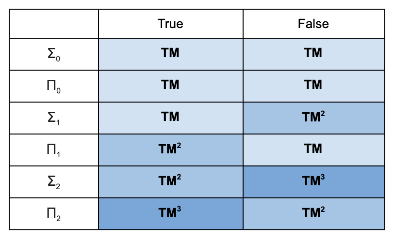
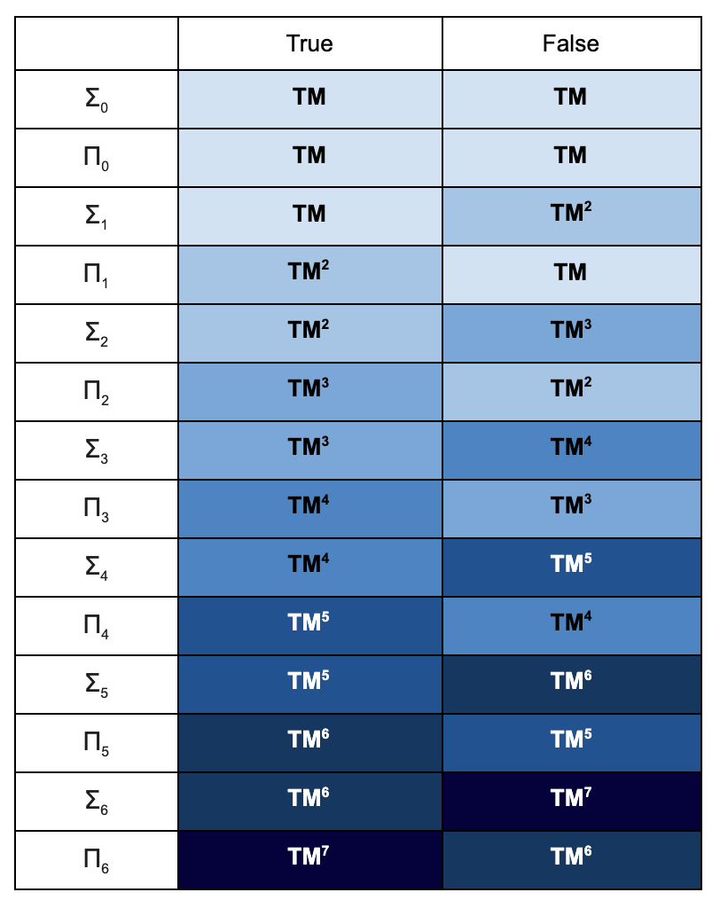
Here’s a summary of what we have so far:
TM = Ordinary Turing Machine TM2 = TM + oracle for TM TM3 = TM + oracle for TM2
The table shows what type of machine suffices to decide the truth value of a sentence, depending on where on the arithmetic hierarchy the sentence falls and whether the sentence is true or false.
We’re now ready to generalize. In general, Σn sentences start with a block of existential quantifiers, and then alternate between blocks of existential and universal quantifiers n – 1 times before ending in a Σ0 sentence. Πn sentences start with a block of universal quantifiers, alternates quantifiers n – 1 times, and then ends in a Σ0 sentence. And as you move up the arithmetic hierarchy, it requires more and more powerful halting oracles to decide whether sentences are true:
If we define Σω to be the union of all the Σ classes in the hierarchy, and Πω the union of the Π classes, then deciding the truth value of Σω ⋃ Πω (the set of all arithmetic sentences) would require a TMω – a Turing machine with an oracle for TM, TM2, TM3, and so on. Thus the theory of true arithmetic (the set of all first-order sentences that are true of ℕ), is not only undecidable, it’s undecidable with a TM2, TM3, and TMn for every n ∈ ℕ. At every level of the arithmetic hierarchy, we get new sentences that are essentially on that level (not just sentences that are superficially on that level in light of their syntactic form, but sentences which, in their simplest possible logically equivalent form, lie on that level).
This gives some sense of just how hard math is. Just understanding the first-order truths of arithmetic requires an infinity of halting oracles, each more powerful than the last. And that says nothing about the second-order truths of arithmetic! That would require even stronger Turing machines than TMω – Turing machines that have halting oracles for TMω, and then TMs with oracles for that, and so on to unimaginable heights (just how high we must go is not currently known).
The Busy Beaver numbers are an undecidable set; if they were decidable, we could figure out BB(n) for each n, enabling us to decide the halting problem. They are also not recursively enumerable, but for a trickier reason. Recursive enumerability would not allow you to figure out BB(n) (as it just gives us the ability to list out the BB numbers in some order, not necessarily in increasing order). But since the sequence is strictly increasing, recursive enumerability would enable us to put an upper bound on BB(n), which is just as good for the purposes of solving the halting problem. Simply enumerate the BB numbers in whatever order your algorithm allows, and once you’ve listed n of them, you know that the largest of those n is at least as big as the BB(n) (after all, it’s a BB number that’s larger than n-1 other BB numbers).
So the Busy Beaver numbers are also not recursively enumerable. But curiously, they’re Turing equivalent to the halting problem, and the halting problem is recursively enumerable. So what gives?
The answer is that the Busy Beaver numbers are co-recursively enumerable. This means that there is an algorithm that takes in a number N and returns False if N is not a Busy Beaver number, and runs forever otherwise. Here’s how that algorithm works:
First, we use the fact that BB(N) is always greater than N. This allows us to say that if N is a Busy Beaver number, then it’s the running time of a Turing machine with at most N states. There are finitely many such Turing machines, so we just run them all in parallel. We wait for N steps, and then see if any machines halt at N steps.
If no machines halt at N steps, then we return False. If some set of machines {M1, M2, …, Mk} halt at N steps, then we continue waiting. If N is not a Busy Beaver number, then for each of these machines, there must be another machine of the same size that halts later. So if N is not a Busy Beaver number, then for each Mi there will be a machine Mi‘ such that Mi‘ has the same number of states as Mi and that halts after some number of steps Ni‘ > N. Once this happens, we rule out Mi as a candidate for the Busy Beaver champion. Eventually, every single candidate machine is ruled out, and we can return False.
On the other hand, if N is a Busy Beaver number, then there will be some candidate machine M such that no matter how long we wait, we never find another machine with the same number of states that halts after it. In this case, we’ll keep waiting forever and never get to return True.
It’s pretty cool to think that for any number that isn’t a Busy Beaver number, we can in principle eventually rule it out. If a civilization ran this algorithm to find the first N busy beaver numbers, they would over time rule out more and more candidates, and after a finite amount of time, they would have the complete list of the first N numbers. Of course, the nature of co-recursive enumerability is that they would never know for sure if they had reached that point; they would forever be waiting to see if one of the numbers on their list would be invalidated and replaced by a much larger number. But in the limit of infinite time, this process converges perfectly to truth.
✯✯✯
Define H to be the set of numbers that encode Turing machines that halt on the empty input, and B to be the set of Busy Beaver numbers. H and B are Turing equivalent. The proof of this is two-part:
H is decidable with an oracle for B
We are given as input a Turing machine M (encoded as some natural number) and asked whether it will halt. We use our oracle for B to find the value of BB(n), where n is the number of states that M has, and run M for BB(n) steps. If M doesn’t halt at this point, then we know that it will never halt and we return False. And if it has already halted, we return True.
2. B is decidable with an oracle for H
We are given as input a number N and asked whether it’s a Busy Beaver number. We collect all Turing machines with at most N states, and apply H to determine which of these halt. We throw out all the non-halting Turing machines and run all the rest. We then run all the remaining Turing machines until each one has halted, noting the number of steps that each runs for and how many states it had. At the end we check if N was the running time of any of the Turing machines, and if so, if there are any other Turing machines with the same number of states that halted later. If so, then we return False, and otherwise we return True.
So H and B have the same Turing degree. And yet B is co-recursively enumerable and H is recursively enumerable (given a Turing machine M, just run it and return True if it ever halts). This is actually not so strange; the difference between recursive enumerability and co-recursive enumerability is not a difference in “difficulty to decide”, it’s just a difference between whether what’s decided is the True instances or the False instances.
As a very simple example of the same phenomenon, consider the set of all halting Turing machines H and the set of all non-halting Turing machines Hc. H is recursively enumerable and Hc is co-recursively enumerable. And obviously given an oracle for either one can also decide the other. More generally, for any set X, consider Xc = {n : n ∉ X}. X and Xc are Turing equivalent, and if X is recursively enumerable then Xc is co-recursively enumerable. What’s more, if X is Σn then Xc is Πn.
In this post you’ll learn about a deep connection between sentences of first order arithmetic and degrees of uncomputability. You’ll learn how to look at a logical sentence and determine the degree of uncomputability of the set of numbers that it defines. And you’ll learn much of the content of and intuitive justification for Post’s theorem, which is perhaps the most important result in computability theory.
The arithmetic hierarchy is a classification system for sets of natural numbers. It relates sentences of Peano arithmetic to degrees of uncomputability. There’s a level of the hierarchy for each natural number, and on each level there are three classes: Σn, Πn, and Δn. Where on the hierarchy a set of naturals lies indicates the complexity of the formulas that define it. Here’s how that works:
Σ0 = Π0 = Δ0
On the zeroth level are all the sets that are definable by a sentence in the language of first-order Peano arithmetic that has no unbounded quantifiers. Examples:
x = 0 (x = 0) ∨ (x = 3) ∨ (x = 200) ∃y < 200 (x = y) ∀y < x ∀z < y (y⋅z = x → z = 1) ∃y < x (x = y + y)
The first two examples have no quantifiers at all. The first, x = 0, is true of exactly one natural number (namely, 0), so the set that it defines is just {0}. The second is true of three natural numbers (0, 3, and 200), so the set it defines is {0, 3, 200}. Thus both {0} and {0, 3, 200} are on the zeroth level of the hierarchy. It should be clear that just by stringing together a long enough disjunction of sentences, we can define any finite set of natural numbers. So every finite set of natural numbers is on the zeroth level of the hierarchy.
The third example has a quantifier in it, but it’s a bounded quantifier. In that sentence, y only ranges over 200 different natural numbers. In some sense, this sentence could be expanded out and written as a long disjunction of the form (x = 0) ∨ (x = 1) ∨ … ∨ (x = 199). It should be easy to see that the set this defines is {0, 1, 2, … 199}.
The fourth example is a little more interesting, for two reasons. First of all, the quantifiers are now bound by variables, not numbers. This is okay, because no matter what value of x we’re looking at, we’re only checking finitely many values of y, and for each value of y, we only check finitely many values of z. Secondly, this formula can be translated as “x is a prime number.” This tells us that the set of primes {2, 3, 5, 7, 11, …} is on the zeroth level of the hierarchy, our first infinite set!
The fifth example also gives us an infinite set; work out which set this is for yourself before moving on!
Notice that each of the sets we’ve discussed so far can be decided by a Turing machine. For each set on the zeroth level, the defining sentence can be written without any quantifiers, involving just the basic arithmetic operations of Peano arithmetic (+, ⋅, and <), each of which is computable. So for instance, we can write an algorithm that decides prime membership for x by looking at the sentence defining the set of primes:
∀y < x ∀z < y (y⋅z = x → z = 1)
for y in range(x):
    for z in range(y):
        if (y⋅z == x) and (z != 1):
            return False
return True
Another example:
(x = 0) ∨ (x = 3) ∨ (x = 200)
if (x = 0) or (x = 3) or (x = 200):
    return True
else:
    return False
Every sentence with only bounded quantifiers can be converted in a similar way to an algorithm that decides membership in the set it defines. We just translate bounded quantifiers as for loops! Thus every set on the zeroth level is decidable. It turns out that every decidable set is also on the zeroth level. We can run the process backwards and, given an algorithm deciding membership in the set, convert it into a sentence of first-order Peano arithmetic with only bounded quantifiers.
On the zeroth level, the three classes Σ0, Π0, and Δ0 are all equal. So every decidable set can be said to be in each of Σ0, Π0, and Δ0. The reason for the three different names will become clear when we move on to the next level of the hierarchy.
Σ1, Π1, Δ1
Entering into the first level, we’re now allowed to use unbounded quantifiers in our definitions of the set. But not just any pattern of unbounded quantifiers, they must all be the same type of quantifier, and must all appear as a block at the beginning of the sentence. For Σ1 sets, the quantifiers up front must all be existential. For example:
∃y (y2 + y + 1 = x) ∃y ∃z (y is prime ∧ z is prime ∧ x = y + z ∧ x is even)
The first defines the infinite set {1, 3, 7, 13, 21, 31, …}, and the second defines the set of all even numbers that can be written as the sum of two primes (whether this includes every even number is unknown!). The shorthand I’ve used in the second sentence is permitted, because we know from the previous section that the sentences “x is prime” and “x is even” can be written without unbounded quantifiers.
It so happens that each of these sets can also be defined by formulas on the zeroth level as well. One easy way to see how is that we can just bound each quantifier by x and everything is fine. But are there any Σ1 sets that aren’t also Σ0?
Yes, there are! Every decidable set is in Σ0, so these examples won’t be as simple. To write them out, I’ll have to use some shorthand that I haven’t really justified:
∃y (the Turing machine encoded by x halts in y steps) ∃y (y Gödel-codes a proof from PA of the sentence Gödel-coded by x)
Both of these rely on the notion of numbers encoding other objects. In the first we encode Turing machines as numbers, and in the second we encode sentences of Peano arithmetic as numbers using Gödel numbering. In general, any finite object whatsoever can be encoded as a natural number, and properties of that object can be discussed as properties of numbers.
Let’s take a close look at the first sentence. The set defined by this sentence is the set of numbers that encode Turing machines that halt. (For readability, in the future I’ll just say “the set of Turing machines such that …” rather than “the set of natural numbers that encode Turing machines with the property …”.) This set is undecidable, by the standard proof of the undecidability of the halting problem. This tells us that the set cannot be defined without any quantifiers!
The second sentence defines the set of natural numbers that encode theorems of PA. Why is this set not decidable? Suppose that it were. Then we could ask “is 0=1 a theorem of PA?” and, assuming the consistency of PA, after a finite amount of time get back the answer “No.” This would allow us to prove the consistency of PA, and crucially, the Turing machine that we use to decide this set could be coded as a number and used by PA to prove the same thing! Then PA would prove its own consistency, making it inconsistent and contradicting our assumption. On the other hand, if PA is inconsistent, then this set actually is decidable, because everything is provable from the axioms of PA and the set of all sentences can be decided! So this is only a good example of “Σ1 but not Σ0” if you have faith in the consistency of PA.
The Σ0 sets were the decidable sets, so what are the Σ1 sets? They are the recursively enumerable sets (also called semi-decidable). These are the sets for which an algorithm exists that takes in an input N and returns True if N is in the set, and runs forever otherwise. And just like before, we can use the sentences of PA to construct such an algorithm! Let’s look at the first example:
∃y (y2 + y + 1 = x)
y = 0
while True:
    if y**2 + y + 1 == x:
        return True
    y += 1
For each unbounded quantifier, we introduce a variable and a while loop that each step increases its value by 1. This program runs until it finds a “yes” answer, and if no such answer exists, it runs forever.
Another example:
∃y (the Turing machine encoded by x halts in y steps)
y = 0
while True:
    if TM(x) halts in y steps:
        return True
    y += 1
I made up some notation here on the fly; TM(x) is a function that when fed a natural number returns the Turing machine it encodes. So what this program does is run TM(x) for increasing lengths of time, returning True if TM(x) ever halts. If TM(x) never halts, then the program runs forever. So this program semi-decides the halting problem.
Moving on to Π1 sets! Σ1 sets were those defined by sentences that started with a block of existential quantifiers, and Π1 sets are defined by sentences that start with a block of unbounded universal quantifiers. For example:
∀y ∀z (x = y⋅z → (y = 1 ∨ x = 1)) ∀y > x ∃z < y (x⋅z = y)
The first example is hopefully clear enough. It defines the set of prime numbers in a similar way to before. The second is meant to be slightly deceiving. That first quantifier might look bounded, until you notice that the variable it supposedly binds ranges over infinitely many values. On the other hand, the second quantifier is genuinely bounded, as for any given y it only ranges over finitely many values. See if you can identify the set it defines.
Both of these sets are in fact also in Σ0. Like with Σ1 sets, it’s difficult to find simple examples of Π1 sets that aren’t also Σ0. Here’s a cheap example:
∀y (the Turing machine encoded by x doesn’t halt in y steps)
This defines the set of non-halting Turing machines. If we were to translate this into a program, it would look something like:
y = 0
while True:
    if TM(x) halts in y steps:
        return False
    y += 1
The difference between this and the earlier example is that this program can only successfully determine that natural numbers aren’t in the set, not that they are in the set. So we can only decide the “no” cases rather than the “yes” cases. Sets like this are called co-recursively enumerable.
So far we have that Σ0 = Π0 = Δ0 = {decidable sets of naturals}, Σ1 = {recursively enumerable sets of naturals}, and Π1 = {co-recursively enumerable sets of naturals}. To finish off level one of the hierarchy, we need to discuss Δ1.
A set is Δ1 if it is both Σ1 and Π1. It can be defined by either type of sentence. In other words, if it is both recursively enumerable (can decide the True instances) and co-recursively enumerable (can decide the False instances). Thus a set is Δ1 if and only if it’s decidable! So every Δ1 set is also a Δ0 set.
A diagram might help at this point to see what we’ve learned:
(“Recursive” is another term for “decidable”)
Σ2, Π2, Δ2
We now enter the second level of the hierarchy. Having exhausted the recursively enumerable, co-RE, and decidable sets, we know that the new sets we encounter can no longer be semi-decided by any algorithms. We’ve thus entered a new realm of uncomputability.
A set is Σ2 if it can be defined by a sentence with a block of ∃s, then a block of ∀s, and finally a Σ0 sentence (free of unbounded quantifiers. Start with some simple examples:
As with any examples you can write as simply as that, the sets these define are also Σ0. So what about sentences that define genuinely new sets that we haven’t seen before? Here’s one:
∃y ∀z (TM(x) doesn’t halt on input y after z steps)
This defines the set of Turing machines that compute partial functions (i.e. functions that run forever on some inputs).
Something funny happens when you start trying to translate this sentence into a program. We can start by translating the existential quantifier up front:
y = 0
while True:
    if ∀z (TM(x) doesn't halt on input y after z steps):
        return True
    y += 1
Now let’s see what it would look like to expand the universal quantifier:
z = 0
while True:
    if TM(x) halts on input y after z steps:
        return False
    z += 1
There’s a problem here. The first program only halts if the second one returns True. But the second one never returns “True”; it’s Π1, co-recursively enumerable! We’ve mixed a recursively enumerable program with a co-recursively enumerable one, and as a result the program we wrote never halts on any input!
This is what happens when we go above the first level of the hierarchy. We’ve entered the realm of true uncomputability.
On the other hand, suppose that we had access to an oracle for the halting problem. In other words, suppose that we are allowed to make use of a function Halts(M, i) that decides for any Turing machine M and any input i, whether M halts on i. Now we could write the following program:
y = 0
while True:
    if not Halts(TM(x), i):
        return True
    y += 1
And just like that, we have a working program! Well, not quite. This program halts so long as its input x is actually in the set of numbers that encode TMs that compute partial functions. If x isn’t in that set, then the program runs forever. This is the equivalent of recursive enumerability, but for programs with access to an oracle for the halting problem!
This is what characterizes Σ2 sets: they are recursively enumerable using a Turing machine with an oracle for the halting problem.
Perhaps predictably, Π2 sets are those that are co-recursively enumerable using a Turing machine with an oracle for the halting problem. Equivalently, these are sets that are definable with a sentence that has a block of ∀s, then a block of ∃s, and finally a Σ0 sentence. An example of such a set is the set of Turing machines that compute total functions. Another is the set of Busy Beaver numbers.
And just like on level one of the hierarchy, the Δ2 sets are those that are both Σ2 and Π2. Such sets are both recursively enumerable and co-recursively enumerable with the help of an oracle for the halting problem. In other words, they are decidable using an oracle for the halting problem. (Notice that again, Δ2 sets are “easier to decide” than Σ2 and Π2 sets.)
The Busy Beaver numbers are an example of a Δ2 set. After all, if one had access to an oracle for the halting problem, they could compute the value of the nth Busy Beaver number. Simply list out all the n-state Turing machines, use your oracle to see which halt, and run all of those that do. Once they’ve all stopped, record the number of steps taken by the longest-running. With the ability to compute the nth Busy Beaver number, we do the following:
n = 1
while True:
    if x == BB(n):
        return True
    n += 1
This returns True for all inputs that are Busy Beaver numbers, but runs forever on those that aren’t. We can fix this with bounded quantifiers: since the Busy Beaver numbers are a strictly increasing sequence, once we’ve reached an n such that x < BB(n), we can return False. This gives us an algorithm that decides the set of Busy Beaver numbers!
In fact, the Busy Beaver numbers are even better than Δ2; they’re Π1, co-recursively enumerable! But that’s a tale for another time.
Σn, Πn, Δn
Perhaps you’re now beginning to see the pattern.
Σ3 sets are those that can be defined by a sentence that has a block of ∃s, then a block of ∀s, then a block of ∃s, and finally a Σ0 sentence. We could more concisely say that Σ3 sets are those that can be defined by a sentence that has a block of ∃s and then a Π2 sentence.
Π3 sets are those definable by a sentence that starts with a block of ∀s, then alternates twice between groups of quantifiers before ending in a sentence with only bound quantifiers.
And Δ3 sets are those that are Σ3 and Π3. If you’ve picked up the pattern, you might guess that the Δ3 sets are exactly those that are decidable with an oracle for the halting problem for Turing machines that have an oracle for the halting problem. The Σ3 sets are those that are recursively enumerable with such an oracle, and the Π3 sets are co-RE with the oracle.
And so on for every natural number.
Σn sets are definable by a sentence that looks like ∃x1 ∃x2 … ∃xk φ(x, x1, x2, …, xk), where φ is Πn-1. Πn sets are definable by a sentence that looks like ∀x1 ∀x2 … ∀xk φ(x, x1, x2, …, xk), where φ is Σn-1. And Δn sets are both Σn and Πn.
At each level of the hierarchy, we introduce new oracle Turing machines with more powerful oracles. We’ll call the Turing machines encountered on the nth level TMns.
Σn sets are recursively enumerable with an oracle for the halting problem for TMns. Πn sets are co-recursively enumerable with an oracle for the halting problem for TMns. Δn sets are decidable with an oracle for the halting problem for TMns.
One might reasonably wonder if at some stage we exhaust all the sets of natural numbers. Or do we keep finding higher and higher levels of uncomputability?
Yes, we do! For each n, Σn is a proper subset of Σn+1 and Πn is a proper subset of Πn+1. One easy argument to see why this must be the case is that there are an uncountable infinity of sets of naturals, and only countably many sets of naturals in each level of the hierarchy. (This is because each level of the hierarchy is equivalent to the sets that are computable/recursively enumerable/co-RE using a TM with a particular oracle, and each TM only computes countably many things.)
This tells us that the hierarchy doesn’t collapse at any finite stage. Each step up, we find new sets that are even harder to decide than all those we’ve encountered so far. But (and now prepare yourself for some wildness) we can make the same cardinality argument about the finite stages of the hierarchy to tell us that even these don’t exhaust all the sets. There are only countably many finite stages of the hierarchy, and each stage contains only countably many sets of naturals!
What this means is that even if we combined all the finite stages of the hierarchy to form one massive set of sets of naturals decidable with any number of oracles for halting problems for earlier levels, we would still have not made a dent in the set of all sets of naturals. To break free of the arithmetic hierarchy and talk about these even more uncomputable levels, we need to move on to talk about the set of Turing degrees, the structure of which is incredibly complex and beautiful.