Credit to Joel David Hamkins, who I heard discussing this paradox on an episode of the podcast My Favorite Theorem.
Define a finite game to be any two-player turn-based game such that every possible playthrough ends after finitely many turns. For example, tic-tac-toe is a finite game because every game ends in at most nine turns.. So is chess with the 50-move-rule enforced (if 50 moves are taken without any pawn advances or captures, then the game ends in a draw). In both these examples, there’s an upper bound to how long the game can last, but this is not required. A game of transfinite Nim would count as finite; every game lasts for only finitely many turns, even though there is no upper bound on the number of turns it takes.
Now, consider the game Hypergame. To play Hypergame, Player 1 begins by choosing any finite game G. Then Player 2 plays the first move of G, Player 1 plays the second move of G, and so on until the game is completed. (Since Player 1 chose a finite game, this will always happen after some finite amount of time.)
Is Hypergame a finite game? Yes, we can easily see that it must be. Whatever game Player 1 chooses will be over after n steps, for some finite n. So that playthrough of Hypergame will have taken n+1 steps.
But if Hypergame is a finite game, then it is a valid choice for the first move of Hypergame! So we can now imagine the following playthrough of Hypergame:
A Troubling Playthrough of Hypergame Player 1: For the finite game that we shall play, I pick Hypergame. Player 2: Hm, okay. So now I’m playing the first move of Hypergame. So I must now choose any finite game. I’ll choose Hypergame! Player 1: Alright so I’m again playing the first move of this new game of Hypergame. I’ll choose Hypergame again. Player 2: And I choose Hypergame again as well. So on forever…
At no point does either player violate the rules of Hypergame. And yet, we ended up with an infinite playthrough of Hypergame, which we proved was impossible! So we have a contradiction. What is the resolution?
✵✵✵
Here’s one possible resolution, analogous to the resolutions of similar set-theoretic paradoxes.
We can think about a game as a directed rooted tree. The vertices of the tree correspond to game states, and the edges correspond to the allowed moves. The root of the tree corresponds to the starting game state, and Player 1 gets to choose which edge to travel along first. From the new vertex, Player 2 decides the next edge to travel along. And so on. The tree’s leaves correspond to ending states of the game, and each leaf is labelled according to which player won in that ending state.
In this framework, what is a finite game? As I defined it above, a finite game is just any directed rooted tree such that every path starting at the root ends at a leaf after passing through finitely many edges. This corresponds perfectly to the idea that every possible playthrough of the game takes only finitely many turns. Notice that a finite game is not necessarily a finite tree! The game tree of a finite game is only finite if it’s also finitely branching. In other words, for a game to have a finite tree requires not just that every playthrough is finitely long, but that each player always has only finitely many choices on their turn.
For instance, the game tree of Hypergame is not a finite tree, because Player 1 has infinitely many possible finite games to choose from on his first turn. How big exactly is the game tree of Hypergame? We know that we have to have a vertex corresponding to the start of any finite game, so it must be at least as large as the set of all finite games. But how large is this set?
This is where we run into problems. The game tree of a finite game can be arbitrarily large. Consider the game which starts by Player 1 choosing any real number and then immediately losing. The height of the game tree is 1, but its width is the cardinality of the continuum. Similarly for any set X we can find a game whose tree has cardinality |X|. This means that there are finite games of arbitrary cardinalities. But then as a corollary to the nonexistence of a largest cardinality, we know that there is no set of all finite games! And this implies that Hypergame has no game tree! More precisely, there is no set corresponding to the game tree of Hypergame as we defined it.
Couldn’t we instead think about Hypergame as a proper class? Sure! But then when we choose a finite game in our first move, we couldn’t be picking Hypergame, as the property “is a finite game” would only apply to sets and not proper classes. This means that we can’t actually select Hypergame as our first move! And so we avoid the paradoxical conclusion that we can keep picking Hypergame ad infinitum.
I find it quite fascinating that the seemingly innocent notion of a finite game can lead us into paradoxes involving proper classes!
Recently I told a friend that I thought ZFC was one of humankind’s greatest inventions. He pointed out that it was pretty bold to claim this about something that most of mankind has never heard of, which I thought was a fair objection. After thinking for a bit, I reflected that the sense of greatness I meant wasn’t really consequentialist, and thus it was independent of how many people know what ZFC is, or even how many people’s lives are affected in any way by it. Instead I intended greatness in a sort of aesthetic and intellectual sense.
The closest analogy to ZFC outside of math is the idea of a “theory of everything” for physics. If we found a theory of everything for physics, it’d likely have a bunch of important practical consequences, and that’d be part of what makes it a great invention. But it would also be a great invention in an intellectual sense, as a discovery of something fundamental and unifying of many seemingly disparate phenomena we observe. This is what ZFC is like: a mathematical theory of everything. One reason this analogy is imperfect is that due to the incompleteness theorems, we know that there can be no “theory of everything” for mathematics. (Any theory of everything will have at least one thing it can’t prove, namely its own consistency.) So ZFC’s greatness can’t come from being a perfect theory of everything, because we know that it is not. Nonetheless, ZFC serves as a foundation for virtually all known mathematics, and this is what I think is so incredible about it.
What does it mean for something to “serve as a foundation” for math? ZFC is a foundation in (at least) three ways: (1) in terms of its ability to define virtually all mathematical concepts, (2) in terms of its structures being rich enough to contain objects that come from virtually all fields of math, and (3) in terms of being an axiom system that suffices to prove virtually every result in known mathematics.
Syntax
Virtually every mathematical concept you can think of has a definition in the language of ZFC. For example, we have definitions for numbers like “π” and “√2”, sets like ℕ and ℝ, algebraic objects like the group S5 and the ring ℚ[x], geometric objects like Platonic solids and differential manifolds, computational objects like Turing machines and cellular automata, and even logical entities like models of first order theories and proofs within formal systems. What makes this especially impressive is the simplicity of the language: it uses nothing besides the basic symbols of first order logic and one binary relation symbol: ∈. So one thing that ZFC teaches us is that virtually every concept in mathematics can be defined just in terms of the set membership relation, and all mathematics can be understood as exploring the properties of this relation.
Semantics
Models of ZFC are insanely richly structured. You can navigate within them to find sets corresponding to every object that mathematicians study. π has a representative set within any model of ZFC, as does the Monster group or the torus. These representative sets are not always perfect: there are models of ZFC where ℝ is countable, for instance. But within the model, they nonetheless share enough similarities with the original objects that virtually everything you can prove about the original object, remains true of the ZFC-representative.
Proof
Finally, ZFC is a computable set of sentences, and we may inquire about what can be proven from it. Keeping up the ambition of the previous two sections, we might want to claim that all mathematical truths can be proven from ZFC. But due to the limitations of first order logic discovered over the last century, we now know that this goal is not achievable. The set of all first order truths of arithmetic is not computable, and so there must be some such truths that aren’t logical consequences of ZFC. Nonetheless, it is commonly claimed that virtually all mathematical truths can be derived from ZFC using the usual proof system for first order logic.
This is especially remarkable given the simplicity of ZFC. I believe that the intuitive content of each axiom could be explained to a smart middle schooler. Additionally, these axioms are extremely intuitively appealing. the most controversial of them has been choice, which is equivalent to the statement that the Cartesian product of non-empty sets is also non-empty. Second most controversial is probably the axiom of infinity, which just says that there’s an infinite set. The rest are even less hard to accept than these.
Now, the fact that you can prove virtually everything from ZFC doesn’t mean that you should. So don’t interpret me as saying that ZFC is of practical use to the daily work of mathematicians trying to prove things outside of set theory and logic. Again, an analogy to physics: we might discover a theory of everything that we know reproduces all the known phenomena of GR and QM, but find that it’s so hard to prove things that we are practically never better off using this theory to calculate things. Nonetheless, ZFC as a theory of everything teaches us that most of math can be understood as conceptually quite simple: the logical consequences of a fairly simple and computable set of sentences about sets. People make a big deal out of Euclid’s axiomatization of geometry, but this is a small feat relative to the axiomatization of all of mathematics.
Metamath
And not only can ZFC prove virtually everything in ordinary mathematics, but ZFC can prove much of what we know in metamathematics and logic itself. When logicians are studying model theory, or even when set theorists are studying ZFC, they are almost always working with ZFC as their meta-theory, meaning that they are making sure that all of their proofs could ultimately be expanded out as ZFC proofs. So the big results of logic, like the completeness theorem, the compactness theorem, the incompleteness theorems, the Löwenheim-Skolem theorems, are all theorems of ZFC.
The fact that ZFC can even talk about these model theoretic notions means that models of ZFC are able to talk about models of ZFC, which is where things get very meta. One can prove that every model of ZFC – every one of these crazily richly-structured universes containing virtually all of mathematics – contains another such model of ZFC. This follows from the reflection theorem, which again can be proven in ZFC!
Hopefully I have now roused enough interest in you to get you to take a look at some of the actual mathematics. You might be curious to know what exactly this theory is. And you’re in luck, it’s simple enough that I can write the whole theory in just nine lines!
Note that with the exception of the final axiom, Choice, the only symbols I’ve used are logical symbols and ∈. I used shorthand for Choice for the sake of readability, but this could be expanded out just like the others. I’m also using a convention where any free variables are considered to be universally quantified over, which shortens things further.
I’ll close with a one-sentence description for each axiom.
Extensionality: No two distinct sets have all the same elements. Pairing: For any two sets, there’s a set containing just those two. Union: The union of any set of sets exists. Powerset: There is a set of all subsets of any set. Specification: For any property Φ and any set x, you can form a set out of just those elements of x with that property. Replacement: For any definable function and any set, the image of that set under the function exists. Infinity: There’s an infinite set. Regularity: Every non-empty set has a member that it shares nothing with. Choice: For any set of nonempty sets, there is a function that picks out one element from each.
The fact that you can prove everything from the infinitude of primes to Fermat’s Last Theorem from just these basic principles, is really quite mind-blowing.
I want to describe a hierarchy of infinitary logics, and show some properties of one of these logics in particular.
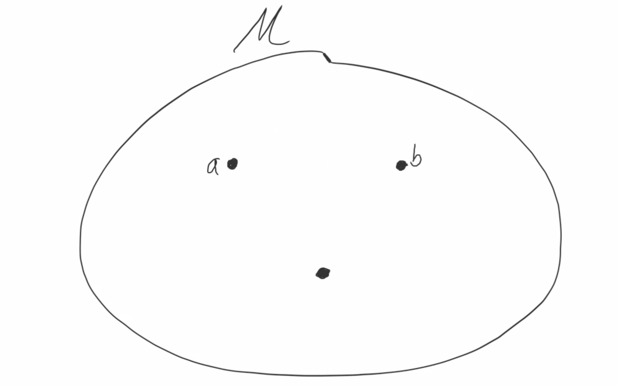
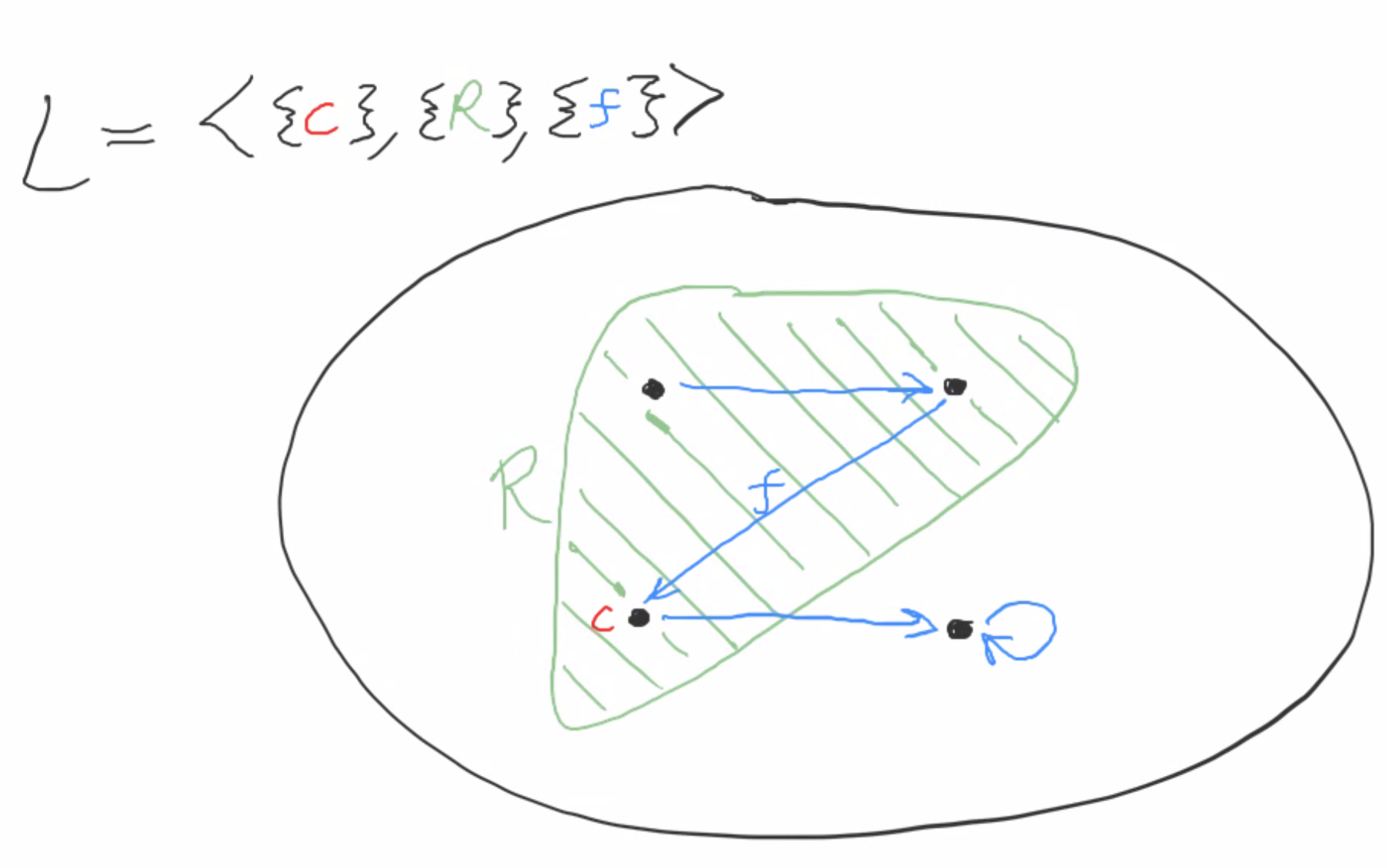
First, a speedy review of first order logic. In the language of first order logic we have access to parentheses {(, )}, the propositional connectives {∧, ∨, ¬, →}, the equals sign {=}, quantifiers {∀, ∃}, and a countably infinite store of variables for quantification over {x1, x2, x3, …}. These are the logical symbols common to any first-order language, but to complete the language we additionally specify a set of constant symbols {c1, c2, c3, …}, function symbols {f1, f2, f3, …}, and relation symbols {R1, R2, R3, …}. These sets can be any cardinality whatsoever. We can then define the set of grammatical sentences (“well-formed formulas”) of this language. We also interpret these symbols in a fairly straightforward way: a first-order structure has a universe of objects, and constants are assigned referents within that universe, function symbols are assigned n-ary functions on the universe, and relation symbols are assigned n-ary relations on the universe.
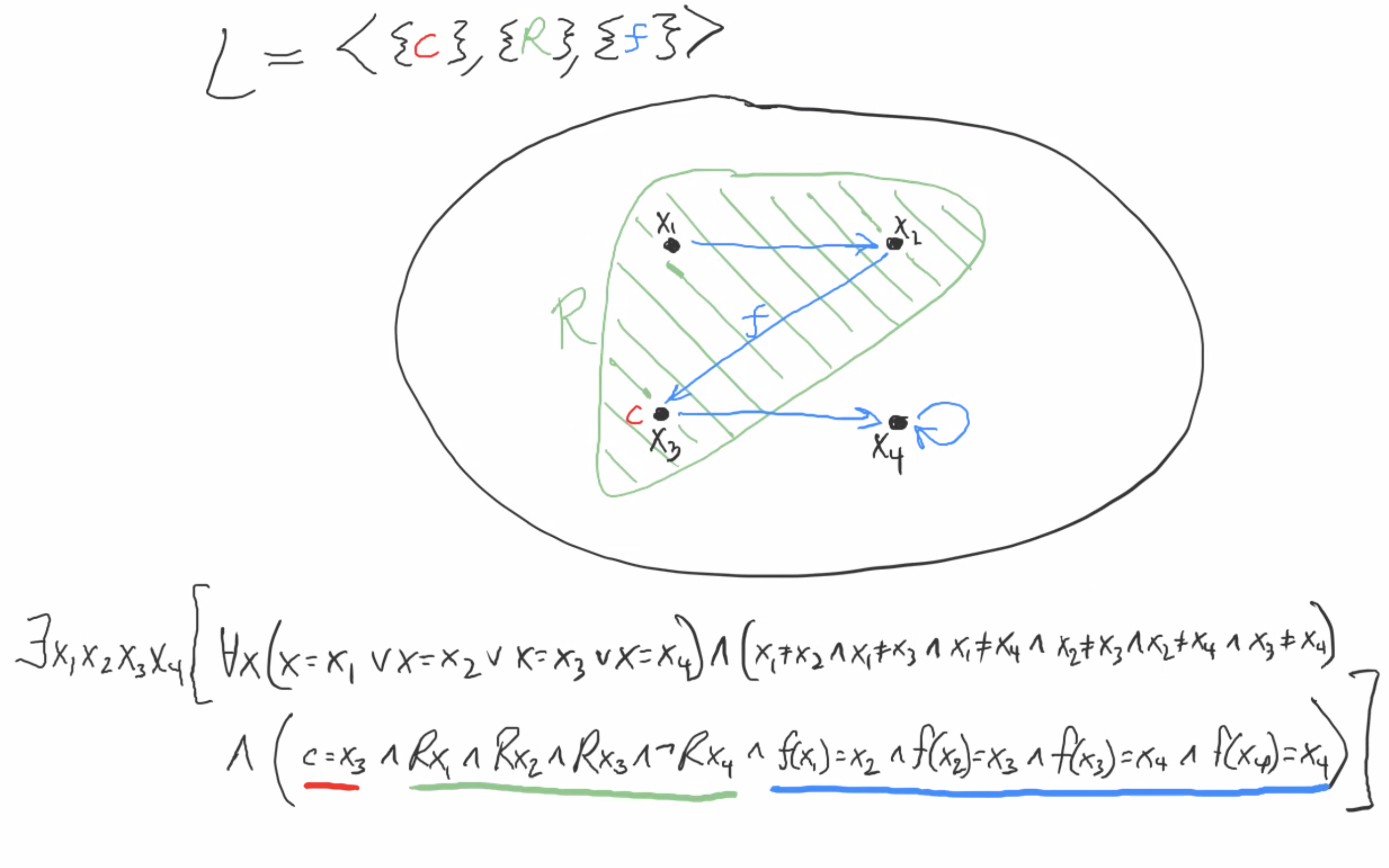
One consequence of the construction is that all of our sentences are finite, which puts an important cap on expressive power. Consider a language of arithmetic with constants for every natural number: {0, 1, 2, 3, …}. We might naturally want to say that the set of constants exhausts all the objects in our universe. But this takes an infinitely long sentence: ∀x (x=0 ∨ x=1 ∨ x=2 ∨ x=3 ∨ …). You might think you could be clever and find a finite expression of this idea, but it turns out that you can’t. (This is a consequence of Gödel’s first incompleteness theorem.)
So a natural extension of first-order-logic is to allow infinitely long sentences. For any two cardinal numbers α and β, define Lα,β to be first-order logic, but with conjunctions of any length < α allowed and blocks of quantifiers of any length < β. (Note that infinite conjunctions implies infinite disjunctions as well.) For example, Lω,ω is ordinary first-order logic: conjunctions and quantifier blocks of any finite length. Lω1,ω is first-order logic plus countably infinite conjunctions, but only finite quantifiers. Lω,ω1 has finite conjunctions but countably infinite quantifiers. Question: what logic is this equivalent to?
Notice that countably infinitely many quantifiers use countably infinitely many variables, but if you only have finite conjunctions you can only use finitely many of them. So this ends up being equivalent to Lω,ω. For this same reason, if β > α then Lα,β is no different from Lα,α.
Lω1,ω is especially interesting to logicians, because it’s significantly stronger than first-order logic, but not so much stronger as to lose all nice proof-theoretic properties. In particular, there’s a sound and complete proof system for Lω1,ω! It’s also quite simple: just the FOL proof system plus one new axiom and one infinitary deduction rule:
New axiom For any m ∈ ω and any set of sentences {φn | n ∈ ω}, ∧n∈ω φn → φm
New inference rule φ0, φ1, φ2, … ⊢ ∧n∈ω φn
If we allow deductions of any countably infinite (successor) ordinal type, then we get a sound and complete proof system. This means that for any countable set of Lω1,ω-sentences Σ and any Lω1,ω-sentence φ, you can deduce φ from Σ just in case Σ actually (ω1,ω)-logically implies φ.
Infinite conjunctions give you a massive boost in expressive power going from FOL to Lω1,ω. You can categorically define the natural numbers: Take Peano arithmetic and add to it the axiom: ∀x ∨n∈ω (x = n). See why this works? We’ll refer back to this theory as PA*.
So Lω1,ω is powerful enough to be able to categorically define the natural numbers. We might wonder if we can also categorically define all other countable structures. It turns out that while we can’t do that, we can do something slightly weaker. For any countable structure, there’s a single Lω1,ω-sentence that defines it up to isomorphism among countable structures. The complexity of this sentence is a way of measuring the complexity of the structure, and has close connections to other measures of structure complexity. (The key word to learn more about this is Scott rank.)
What else can you do with Lω1,ω? Here’s something really cool: Tarski’s theorem on the undefinability of truth tells us that in first-order logic you cannot define a truth predicate. But in Lω1,ω, you can! Take a countable first-order language L. Add on the language of arithmetic (0, S, +, ×, ≤) to L. L is still countable, so enumerate all its sentences {φ1, φ2, φ3, …}. Now, the sentence Tr(x) := ∨n∈ω (x=n & φn) is a truth predicate: for any n, if φn is true then Tr(n) is true and if φn is false then Tr(n) is false.
You can express the idea that “infinitely many things satisfy φ(x)” with the following sentence:
The first line says “there’s at least two things satisfying φ”, the second says “there’s at least three things satisfying φ”, and so on forever.
Finally, unlike FOL, Lω1,ω is not compact. This means that there are sets of sentences without models, where every finite subset has a model. But it’s actually even worse than that! Lω1,ω is strongly non-compact. You can have an unsatisfiable set of sentences, every countable subset of which has a model! Once again, this pretty remarkable fact has a simple proof:
Take the language of Peano arithmetic and add on ℵ1-many constant symbols: {cα | α < ω1}. Now add to PA* the set of sentences {cα ≠ cβ | α ≠ β, both in ω1}. Let’s call this theory Σ. Every countable subset of Σ has a model, but Σ itself doesn’t. You can always take countably many constant symbols and assign them distinct referents in ℕ such that some natural numbers are left out. However, you can’t assign uncountably many distinct referents in ℕ while still leaving out some natural numbers, by a simple cardinality argument.
There’s an interesting twist here: Consider the set of sentences {cα ≠ cβ | α ≠ β, both < ω1CK} ⊂ Σ, where ω1CK is the Church-Kleene ordinal, the smallest uncomputable ordinal. ω1CK is countable, so this is a countable set of sentences. This set of sentences has a model, but to obtain it you must choose a bijection from the set of constants {cα | α < ω1CK} to the natural numbers. By the definition of ω1CK, this bijection is uncomputable! There are uncountably many countable ordinals above ω1CK (there are countably many computable ordinals, and uncountably many countable ordinals), so while every countable subset of Σ has a model, uncountably many of these models will be uncomputable!
Now the pieces are all in place to start applying forcing to prove some big results. Everything that follows assumes the existence of a countable transitive model M of ZFC.
First, a few notes on terminology.
The language of ZFC is very minimalistic. All it has on top of the first-order-logic connectives is a single binary relation symbol ∈. Nonetheless, people will usually talk about theorems of ZFC as if it has a much more elaborate syntax, involving symbols like ∅ and ω and ℵ1 and terms like “bijection” and “ordinal”. For instance, the Continuum Hypothesis can be written as “There’s a bijection between 𝒫(ω) and ℵ1“, which is obviously using much more than just ∈. But these terms are all simply shorthand for complicated phrases in the primitive language of ZFC: for instance a sentence “φ(∅)” involving ∅ could be translated as “∃x (∀y ¬(y ∈ x) ∧ φ(x))”, or in other words “there’s some set x that is empty and φ(x) is true”.
Something interesting goes on when considering symbols like ∅ and ω and ℵ1 that act like proper names. Each name picks out a unique set, but for some of these names, the set that gets picked out differs in different models of ZFC. For example, the interpretation of the name “ℵ1” is model-relative; it’s meant to be the first uncountable cardinal, but there are countable models of ZFC in which it’s actually only countably large! If this makes your head spin, it did the same for Skolem: you can find more reading here.
On the other hand, the name “∅” always picks out the same set. In every model of ZFC, ∅ is the unique set that contains nothing at all. When a name’s interpretation isn’t model-relative, it’s called absolute. Examples include “∅” and “1,729”. When a name isn’t absolute, then we need to take care to distinguish between the name itself as a syntactic object, and the set which it refers to in a particular model of ZFC. So we’ll write “ℵ1” when referring to the syntactic description of the first uncountable cardinal, and ℵ1M when referring to the actual set that is picked out by this description in the model M.
With that said, let’s talk about a few names that we’ll be using throughout this post:
In M, ω is the conventional name for the set that matches the description “the intersection of all inductive sets”, where inductive sets are those that contain the ordinal 0 and are closed under successor. In any transitive model of ZFC like M, ω is exactly ℕ, the set of natural numbers. Since we’re restricting ourselves to only considering transitive models, we can treat ω as if it’s unambiguous; its interpretation won’t actually vary across the models we’re interested in.
ω1 corresponds to the description “the smallest uncountable ordinal”. This description happens to perfectly coincide with the description “the first uncountable cardinal” in ZFC, which has the name ℵ1. But unlike with ω, different transitive models pick out different sets for ω1 and ℵ1. So in a model M, we’ll write ω1M for the set that M believes to be the smallest uncountable ordinal and ℵ1M for the first uncountable cardinal.
ω2 is the name for the first ordinal for which there’s no injection into ω1 (i.e. the first ordinal that’s larger than ω1). Again, this is not absolute: ω2M depends on M (although again, ω2M is the same as ℵ2M no matter what M is). And in a countable model like those we’ll be working with, ω2M is countable. This will turn out to be very important!
𝒫(ω) is the name for the the set that matches the description “the set of all subsets of ω”. Perhaps predictably at this point, this is not absolute either. So we’ll have to write 𝒫(ω)M when referring to M’s version of 𝒫(ω).
Finally, ZFC can prove that there’s a bijection from 𝒫(ω) to ℝ, meaning that this bijection exists in every model. Thus anything we prove about the size of 𝒫(ω) can be carried over to a statement about the size of ℝ. Model-theoretically, we can say that in every model M, |𝒫(ω)M| = |ℝM|. It will turn out to be more natural to prove things about 𝒫(ω) than ℝ.
Okay, we’re ready to make the continuum hypothesis false! We’ll do this by choosing a partially ordered set (P, ≤) whose extension as a Boolean algebra (B, ≤) has the property that no matter what M-generic filter G in B you choose, M[G] will interpret its existence as proof that |𝒫(ω)| ≥ ℵ2.
Making |𝒫(ω)| ≥ ℵ2
Let P = { f ∈ M | f is a finite partial function from ω2M × ω to {0,1} }. Let’s have some examples of elements of P. The simplest is the empty function ∅. More complicated is the function {((ω+1, 13), 1)}. This function’s domain has just one element, the ordered pair (ω+1, 13), and this element is mapped to 1. The function {((14, 2), 0), ((ω1M•2, 2), 1)} is defined on two elements: (14, 2) and (ω1M•2, 2). And so on.
We’ll order P by reverse inclusion: f ≤ g iff f ⊇ g. Intuitively, f ≤ g if f is a function extension of g: f is defined everywhere that g is and they agree in those places. For instance, say f = {((ω, 12), 0)}, g = {((ω, 12), 0), ((13, 5), 1)}, h = {((ω, 12), 1)}, and p = {((ω, 11), 1)}. Check your understanding by verifying that (1) g ≤ f, (2) f and h are incomparable and have no common lower bound, and (3) f and p are incomparable but do have a common lower bound (what is it?).
The empty function ∅ is a subset of every function in P, meaning that ∅ is bigger than all functions. Thus ∅ is the top element of this partial order. And every f in P is finite, allowing a nice visualization what the partial order (P, ≤) looks like:
Now, G will be an M-generic ultrafilter in the Boolean extension (B, ≤) of (P, ≤). G is the set that we’re ultimately adding onto M, so we want to know some of its properties. In particular, how will we use G to show that |𝒫(ω)| = ℵ2?
What we’re going to do is construct a new set out of G as follows: first take the intersection of P with G. (remember that G is an ultrafilter in B, so it doesn’t only contain elements of P). P⋂G will be some set of finite partial functions from ω2M × ω to {0,1}. We’ll take the union of all these functions, and call the resulting set F. What we’ll prove of F is the following:
(1) F := ⋃(P⋂G) is a total function from ω2M × ω to {0,1} (2) For every α, β ∈ ω2M, F(α, •) is a distinct function from F(β, •).
A word on the second clause: F takes as input two things: an element of ω2M and an element of ω. If we only give F its first input, then it becomes a function from ω to {0,1}. For α ∈ ω2M, we’ll give the name Fα to the function we get by feeding α to F. Our second clause says that all of these functions are pairwise distinct.
Now, the crucial insight is that each Fα corresponds to some subset of ω, namely {n ∈ ω | Fα(n) = 1}. So F defines |ω2M|-many distinct subsets of ω. So in M[G], it comes out as true that |𝒫(ω)M| ≥ |ω2M|. It’s also true in M[G] that |ω2M| = ℵ2M, and so we get that |𝒫(ω)M| ≠ ℵ1M. This is ¬CH!
Well… almost. There’s one final subtlety: |𝒫(ω)M| ≠ ℵ1M is what ¬CH looks like in the model M. For ¬CH to be true in M[G], it must be that that |𝒫(ω)M[G]| ≠ ℵ1M[G]. So what if |𝒫(ω)M| ≠ |𝒫(ω)M[G]|, or ℵ1M ≠ ℵ1M[G]? This would throw a wrench into our proof: it would mean that M[G] believes that M’s version of 𝒫(ω) is bigger than M’s version of ℵ1, but M[G] might not believe that its own version of 𝒫(ω) is bigger than its version of ℵ1. This is the subject of cardinal collapse, which I will not be going into. However, M[G] does in fact believe that 𝒫(ω)M = 𝒫(ω)M[G] and that ℵ1M = ℵ1M[G].
Alright, so now all we need to do to show that M[G] believes ¬CH is to prove (1) that F is a total function from ω2M × ω to {0,1}, and (2) that for every α, β ∈ ω2M, Fα is distinct from Fβ. We do this in three steps:
F is a function.
F is total.
For every α, β ∈ ω2M, Fα is distinct from Fβ.
Alright so how do we know that F is a function? Remember that F = ⋃(P⋂G). What if some of the partial functions in P⋂G are incompatible with each other? In this case, their union cannot be a function. So to prove step 1 we need to prove that all the functions in P⋂G are compatible. This follows easily from two facts: that G is an ultrafilter in B and P is dense in B. The argument: G is an ultrafilter, so for any f, g ∈ P there’s some element f∧g ∈ B that’s below both f and g. All we know about f∧g is that it’s an element of B, but we have no guarantee that it’s also a member of P, our set of partial functions. In other words, we can’t say for sure that f∧g is actually a partial function from ω2M × ω to {0,1}. But now we use the fact that P is dense in B! By the definition of density, since f∧g is an element of B, P must contain some h ≤ f∧g. Now by transitivity, h ≤ f and h ≤ g. So f and g have a common function extension, meaning they must be compatible functions! Pretty magical right?
So F is a function. But how do we know that it’s total? We prove this by looking closely at the dense subsets of P. In particular, for any α ∈ ω2M and any n ∈ ω, define Dα,n := {f ∈ P | (α, n) ∈ dom(f)}. This is a dense subset of P. Why? Well, regardless of what α and n are, any function f in P is either already defined on (α, n), in which case we’re done, or it’s not, in which case f has a function extension with (α, n) in its domain. So from any element of P, you can follow the order downwards until you find a function with (α, n) in its domain. Since Dα,n is dense in P and G is M-generic, G must have some element in common with Dα,n. Thus G contains an element f of P that has (α, n) in its domain. This f is one of the functions that we union over to get F, so F must have (α, n) in its domain as well! And since α and n were totally arbitrary, F must be total.
Finally, why are the “Fα”s pairwise distinct? Again we construct dense subsets for our purposes: for any α, β ∈ ω2M, define Dα,β := {f ∈ P | fα ≠ fβ}. This is clearly dense (you can always extend any f in P to make fα and fβ disagree somewhere). So G contains an element f of P for which fα ≠ fβ. And thus it must also be true of F that Fα ≠ Fβ!
And we’re done! We’ve shown that once we add G to M, we can construct a new set F = ⋃(P⋂G) such that F encodes |ω2M|-many distinct subsets of ω, and thus that M[G] ⊨ |𝒫(ω)| ≥ ℵ2.
Making |𝒫(ω)| ≥ ℵ420
What’s great is that this argument barely relied on the “2” in ω2M. We could just as easily have started with P = {f ∈ M | f is a finite partial function from ω420M × ω to {0,1}}, constructed an M-generic filter G in the Boolean extension of P, then defined F to be ⋃(P⋂G).
G is still an ultrafilter in B and P is still dense in B, so F is still a function.
Dα,n := {f ∈ P | (α, n) ∈ dom(f)} is still a dense subset of P for any α ∈ ω420M and any n ∈ ω, so F is still total.
And Dα,β := {f ∈ P | fα ≠ fβ} is still a dense subset of P for any α, β ∈ ω420M, so all the “Fα”s are pairwise distinct.
And now F encodes |ω420M|-many distinct subsets of ω! The final step, which I’m going to skip over again, is showing that M[G] believes that |ω420M| = |ω420M[G]|, i.e. that cardinal collapse doesn’t occur.
And there we have it: this choice of P gives us a new model M[G] of ZFC that believes that |𝒫(ω)| ≥ ℵ420! Note how easy and quick this argument is now that we’ve gone through the argument for how to make M[G] believe |𝒫(ω)| ≥ ℵ2. This is a great thing about forcing: once you really understand one application, other applications become immensely simpler and easier to understand.
Making |𝒫(ω)| = ℵ1
Okay, we’ve made CH false. Now let’s make it true! This time our choice for (P, ≤) will be the following:
P = {f ∈ M | f is an M-countable partial function from ω1M to 𝒫(ω)M}. Once more we order by reverse inclusion: f ≤ g iff f ⊇ g.
A crucial thing to notice is that I’ve merely required the functions in P to be M-countable, rather than countable. For a set to be M-countable is for there to exist an injection in M from set to ω. Any M-countable set is countable, but some countable sets may not be M-countable (like M itself!). In particular, we know that ω1M is actually a countable set, meaning that if we required true countability instead of just M-countability, then P would include some total functions! But M has no injection from ω1M to ω, so no function in P can be total. This will be important in a moment!
We get our M-generic ultrafilter G and define F := ⋂(P⋂G). Now we want to show that F is a total and surjective function from ω1M to 𝒫(ω). As before, we proceed in three steps:
F is a function
F is total
F is surjective
Step 1: G is an ultrafilter and P is dense in G, so the same argument works to show that all elements of P⋂G are compatible: (1) ultrafilter implies that any f, g in P⋂G have a least upper bound f∧g in B, (2) density of P in G implies that f∧g has a lower bound h in P, so (3) f and g have a common function extension . Thus F is a function.
Step 2: Dα := {f ∈ P | α ∈ dom(f)} is dense in P for any α ∈ ω1M, so F is total.
Step 3: DA := {f ∈ P | A ∈ image(f)} is dense in P for any A ∈ 𝒫(ω)M. Why? No f in P is total, so any f in P can be extended by adding one more point (α, A) where α ∉ dom(f). Thus A ∈ image(F) for any A ∈ 𝒫(ω), so F is surjective.
So F is a total surjective function from ω1M to 𝒫(ω)M, meaning that in M[G] it’s true that |𝒫(ω)M| ≤ ℵ1M. And since ZFC proves that |𝒫(ω)| > ℵ0, it follows that M[G] ⊨ |𝒫(ω)| = ℵ1.
You might have noticed that each of these arguments could just as easily have been made if we had started out with defining P as the finite partial functions in M from ω1M to 𝒫(ω)M. This is true! If we had done this, then we still would have ended up proving that F was a total surjective function from ω1M to 𝒫(ω)M, and therefore that |𝒫(ω)M| = ℵ1M. However, this is where cardinal collapse rears its ugly head: the final step is to prove that |𝒫(ω)M| = |𝒫(ω)M[G]| and that ℵ1M = ℵ1M[G]. This requires that P be the countable partial functions rather than just the finite ones.
And with that final caveat, we see that M[G] believes that |𝒫(ω)| = ℵ1.
Making |𝒫(ω)| ≤ ℵ314
Let P = {f ∈ M | f is an M-countable partial function from ω314M to 𝒫(ω)} and order by reverse inclusion: f ≤ g iff f ⊇ g.
⋂(P⋂G) is again a total and surjective function from ω314M to 𝒫(ω), following the exact same arguments as in the previous section. Cardinal collapse doesn’t occur here either, so M[G] believes that |𝒫(ω)| ≤ ℵ314.
✯✯✯
We’ve proven the independence of the Continuum Hypothesis from ZFC! We’ve done more: we’ve also shown how to construct models of ZFC in which we have lots of control over the size of 𝒫(ω). Want a model of ZFC in which |𝒫(ω)| is exactly ℵ1729? Just force with the right P and you’re good to go! There’s something a bit unsatisfactory about all this though, which is that in each application of forcing we’ve had to skim over some details about cardinal collapse that were absolutely essential to the proof going through. I hope to go into these details in a future post to close these last remaining gaps.
Forcing is a set-theoretic technique developed by Paul Cohen in the 1960s to prove the independence of the Continuum Hypothesis from ZFC. He won a Fields Medal as a result, and to this day it’s the only Fields Medal to be awarded for a work in logic. It’s safe to say that forcing is one of the most powerful techniques that set theorists have at their disposal as they explore the set theoretic multiverse.
Forcing has an intimidating reputation, which is somewhat deserved. The technique involves many moving parts and it takes some time to see how they all fit together. I found these three resources to be excellent for learning the basics of the technique:
Each of these sources takes a slightly different approach, and I think that they complement each other quite well. I’ve produced a high-level outline of the argument for why forcing works, as well as how to use forcing to prove the independence of the CH. I don’t feel quite competent to present all of forcing from the ground up, so this outline is not meant to be self-contained. In particular, I’m gonna assume you’re familiar with the basics of first order logic and ZFC and are comfortable with Boolean algebras. I’m also going to skim over the details of cardinal collapse, which are still fairly opaque to me.
Forcing in 5 lines!
Fix a countable transitive model M ⊨ ZFC and a Boolean algebra (B, ≤) ∈ M.
Define MB := { f ∈ M | f: MB ⇀ B } ⊆ M.
Choose an M-generic ultrafilter G ⊆ B.
For every n in MB, define valG(n) := { valG(m) | (m, b) ∈ n for some b in G }.
Define M[G] := { valG(n) | n ∈ MB }. This is a countable transitive model of ZFC containing all of M as well as G!
We start with a countable transitive model M of ZFC, and then construct a larger countable transitive model M[G] of ZFC that contains a new set G. Let me say a few words on each step.
Step 1 1. Fix a countable transitive model M ⊨ ZFC and a Boolean algebra (B, ≤) ∈ M.
There’s not much to say about Step 1. I suppose it’s worth noting that we’re assuming the existence of a countable transitive model of ZFC, meaning that the results of forcing are all conditioned not just on the consistency of ZFC, but on the existence of transitive models of ZFC, which is significantly stronger. (The existence of countable transitive models is no stronger than the existence of transitive models, by the downwards Lowenheim-Skolem theorem.)
Moving on!
Step 2 2. Define MB := { f ∈ M | f: MB ⇀ B }
MB is sometimes called a Boolean-valued model of ZFC. The elements of MB are called “B-names” or “B-valued sets” or just “B-sets” (as I’ll call them). These B-sets are partial functions in M that go from MB to B. “Huh? Hold on,” I hear you saying, “Isn’t that a circular definition?”
It might look circular, but it’s not; it’s inductive. First of all, regardless of what MB is, the empty set counts as a partial function from MB to B: all its inputs are in MB, all its outputs are in B, and no input gets sent to multiple outputs! ∅ is also in M, so ∅ is an element of MB. But now that we know that ∅ is in MB, we can also construct the function {(∅, b)} for each b in B. This satisfies the criterion of “being a partial function from MB to B”, and it is in M because B is in M. So for any b in B, {(∅, b)} is in MB. And now we can construct more partial functions with these new elements of MB, like {(∅, b), ({(∅, b’)}, b’’)} and so on.
If you’re still not convinced that the definition of MB is sensible, we can define it without any apparent circularity, making the induction explicit:
V0 = ∅
Vα+1 = { f ∈ M | f is a partial function from Vα to B } for any ordinal α in M.
Vλ = ⋃{Vα | α ∈ λ} for any limit ordinal λ in M.
Finally, MB = ⋃{Vα | α ∈ M}.
Okay, so now we know the definition of MB. But what is it? How do we intuitively think about the elements of MB? One way is to think of them as “fuzzy sets”, sets that contain each other to varying degrees. In this way of seeing things, the Boolean algebra B is our extension of the trivial Boolean algebra {True, False} to a more complicated Boolean algebra that allows intermediate truth values as well. So for instance, of the B-set {(∅, b)} we can say “it contains ∅ to degree b, and contains nothing else”. Of the B-set {(∅, b), ({(∅, b’)}, b’’)} we may say “it contains ∅ to degree b, and contains [the set that contains ∅ to degree b’] to degree b’’, and nothing else.” And so on.
Every Boolean algebra has a top element ⊤ corresponding to “definite truth” and a bottom element ⊥ corresponding to “definite falsity”, so our B-sets don’t have to be entirely fuzzy. For instance the B-set {(∅, ⊤)} definitely contains ∅ and definitely doesn’t contain anything else. It can be thought of as intuitively similar to the set {∅} in M. And the B-set {(∅, ⊥)} definitely doesn’t contain ∅, or anything else for that matter. This brings up an interesting question: how is the B-set {(∅, ⊥)} any different from the B-set ∅? They have the same intuitive properties: both contain nothing (or said differently, contain each thing to degree ⊥). Well that’s right! You can think of {(∅, ⊥)} and ∅ as two different names for the same idea. They are technically distinct as names, but in Steps 3 and 4 when we collapse MB back down to an ordinary model of ZFC, the distinction between them will vanish. (The details of how exactly we assign B-values to sentences about MB are interesting in their own right, and might deserve their own post.)
So intuitively what we’ve done is take our starting model M and produce a new structure that looks a lot like M in many ways except that it’s highly ambiguous: in addition to all the old sharp sets we have all these new fuzzy sets that are unsure about their members. In the next two steps we collapse all this ambiguity back down, erasing all of the fuzziness. It turns out that there are many ways to collapse the ambiguity (one for each ultrafilter in B in fact!), but we’ll want to choose our ultrafilter very carefully so that we (1) don’t end up back where we started, (2) end up with a model of ZFC, and (3) end up with an interesting model of ZFC.
Step 3 3. Choose an M-generic ultrafilter G ⊆ B.
There’s some terminology here that you might be unfamiliar with.
Firstly, what’s an ultrafilter? It’s a nonempty proper subset of B that’s closed upwards, closed under intersection, and contains one of b or ¬b for each b in B. I talked about ultrafilters here in the context of power sets, but it generalizes easily to Boolean algebras (and there are some pretty pictures to develop your intuitions a bit).
Okay, so that’s what ultrafilters are. What is it to be a generic ultrafilter? A generic ultrafilter is one that intersects every dense subset of B. What’s a dense subset of B? A dense subset of a Boolean algebra (B, ≤) is any subset of B\{⊥} that lower-bounds all of B\{⊥}. In other words, D is a dense subset of B if for every element of B\{⊥} there’s a lower element of D. Intuitively, D is like a foundation that the rest of B\{⊥} rests upon (where “upwards” corresponds to “greater than”). No matter where you are in B\{⊥}, you can follow the order downwards and eventually find yourself at an element of D. And a generic ultrafilter is an ultrafilter that shares something in common with each of these foundational subsets.Why have we excluded the bottom element of B, ⊥? If we hadn’t done so then the dense subsets would just be any and all sets containing ⊥! Then any generic ultrafilter would have to contain ⊥, but this is inconsistent with the definition of an ultrafilter!
Finally, what’s an M-generic ultrafilter? Recalling that a generic ultrafilter has to intersect every dense subset of B, an M-generic ultrafilter only needs to intersect every dense subset of B that’s in M.
I hear a possible objection! “But you already told us that B is in M! And since ZFC has the power set axiom, don’t we know that M must also contain all of B’s subsets? If so then M-genericity is no different from genericity!” The subtlety here is that the power set axiom guarantees us that M contains a set 𝒫(B) that contains all the subsets of B that are in M. Nowhere in ZFC is there a guarantee that every subset of B exists, and in fact such a guarantee is not possible in any first-order theory whatsoever! (Can you see how this follows from the downward Lowenheim-Skolem theorem?) The power set axiom doesn’t create any subsets of B, it merely collects together all the subsets of B that already exist in M.
Now, why do we care about G being M-generic? A few steps down the line we’ll see why M-genericity is such an important property, but in all honesty my intuition is murky here as to how to motivate it a priori. For now, take it on faith that M-genericity ends up being exactly the right property to require of G for our purposes. We’ll end up making extensive use of the fact that G intersects every dense subset of B in M.
Very keen readers might be wondering: how do we know that an M-generic ultrafilter even exists? This is where the countability of M saves us: since M is countable, it only contains countably many dense subsets of B: (D0, D1, D2, …). We construct G as follows: first we choose any b0 ∈ D0. Then for any n ∈ ℕ, since Dn+1 is dense in B, we can find a dn+1 ∈ Dn+1 such that dn+1 ≤ dn. Now we have an infinite descending chain of elements from dense subsets. Define G to be the upwards closure of {dn | n ∈ ℕ}, i.e. G = {b ∈ B | b ≥ dn for some n ∈ ℕ}. This is M-generic by construction, and it’s an ultrafilter: for any b ∈ B, either {b’ ∈ B | b’ ≤ b} or {b’ ∈ B | b’ ≤ ¬b} is dense, implying that G contains either b or ¬b. (Convince yourself that it’s also closed upwards and under ∧.)
Really important note: this proof of G’s existence relies on the countability of M. But from M’s perspective, it isn’t countable; i.e. M doesn’t believe that there’s a bijection that puts each set in correspondence with an element of omega. So M can’t prove the existence of G, and in fact G is a set that doesn’t exist within M at all.
Step 4 4. For every n in MB, define valG(n) := {valG(m) | (m, b) ∈ n for some b in G}.
Ok, next we use G to define a “valuation function” valG(•). This function takes the B-sets created in Step 2 and “collapses” them into ordinary sets. It’s defined inductively: the G-valuation of a B-set n is defined in terms of the G-valuations of the elements of n. (As a side note, the fact that this definition works relies on the transitivity of our starting model! Can you see why?)
Let’s work out some simple examples. Start with n = ∅. Then valG(∅) = {valG(m) | (m, b) ∈ ∅ for some b in G} = ∅, because there is no (m, b) in ∅. Thus G evaluates ∅ as ∅. So far so good! Now for a slightly trickier one: n = {(∅, b)}, where b is some element of B.
valG( {(∅,b)} ) = {valG(m) | (m, b) ∈ {(∅, b)} for some b in G} = {valG(m) | m = ∅ & b ∈ G}
There are two cases: either b is in G or b is not in G. In the first case, {(∅, b)} is evaluated to be {∅}. In the second, {(∅,b)} is evaluated to be {}. What’s the intuition here? G is a subset of B, and we can think of it as a criterion for determining which Boolean values will be collapsed to True. And since G is an ultrafilter, every Boolean value will either be collapsed to True (if b ∈ G) or to False (if ¬b ∈ G). Recall that we thought of {(∅, b)} as a B-set that “contained ∅ to degree b”. Our G-evaluation of this set removed all fuzziness: if b was included in G then we evaluate {(∅, b)} as actually containing ∅. And if not, then we said that it didn’t. Either way, all fuzziness has been removed and we’ve ended up with an ordinary set!
The same happens for every B-set. When we feed it into the function valG(•), we collapse all its fuzziness and end up with an ordinary set, whose members are determined by our choice of B.
Step 5 5. Define M[G] := {valG(n) | n ∈ MB}. M[G] is a countable transitive model of ZFC such that M ⊆ M[G] and G ∈ M[G].
Now we simply evaluate all the B-sets and collect them together, and give the result a name: M[G]. This part is easy: the hard work has already been done in defining MB and valG. What remains is to show that this new set is a countable transitive model of ZFC containing all of M as well as G. Let’s do this now.
First of all, why is M[G] countable? Well, M is countable and MB is a subset of M, so MB is countable. And valG is a surjective function from MB into M[G], so |M[G]| ≤ |MB|.
Second, why is M[G] transitive? This follows immediately from its definition: the elements of M[G] are G-valuations, and elements of G-valuations are themselves G-valuations. So elements of elements of M[G] are themselves elements of M[G]. That’s transitivity!
Third, why is M[G] a model of ZFC? Er, we’ll come back to this one.
Fourth, why is M ⊆ M[G]? To show this, we’ll take any arbitrary set x in M and show that it exists in M[G]. To do this, we first define a canonical name for x: a B-set Nx that acts as the surrogate of x in MB. Define Nx to be {(Ny, ⊤) | y ∈ x}. (Make sure that Nx is actually in MB!) What’s the G-valuation of Nx? It’s just x! Here’s a proof by ∈-induction:
First, N∅ = {(Ny,⊤) | y ∈ ∅} = ∅. So valG(N∅) = valG(∅) = {valG(m) | (m, b) ∈ ∅ for some b in G} = ∅.
Now, assume that valG(Ny) = y for every y ∈ x. Then valG(Nx) = {valG(Ny) | (Ny, b) ∈ Nx for some b in G} = {y | (Ny, ⊤) ∈ Nx} = {y | y ∈ x} = x.
Thus by ∈-induction, for all x, valG(Nx) = x.
Finally, why is G ∈ M[G]? We prove this by finding a B-set that G-valuates to G itself. Define A := {(Nb, b) | b ∈ B}. Then valG(A) = { valG(m) | (m, b) ∈ A for some b in G } = {valG(Nb) | b ∈ G} = {b | b ∈ G} = G.
And there it is! We’re done!
Ha ha, tried to pull a fast one on you. We still have one crucial step remaining: proving that M[G] is actually a model of ZFC! As far as I know, there’s no concise way to do this… you have to actually go through each axiom of ZFC and verify that M[G] satisfies it. I’m not going to do that here, but I will provide proofs of four axioms to give you a flavor.
Infinity: M contains a set I satisfying the axiom of infinity and M ⊆ M[G]. So I ∈ M[G], and it still satisfies infinity (still contains ∅ and is closed under successor).
Pairing: Let x and y be any two sets in M[G]. Then for some n1 and n2 in MB, x = valG(n1) and y = valG(n2). Now define n := {(n1, ⊤), (n2, ⊤)} ∈ MB. Then valG(n) = {x, y}.
Union: Let x be any element of M[G]. Since M[G] is transitive, every element y of an element of x is in M[G]. So for each such y there’s a B-set ny such that valG(ny) = y. Define n := {(ny,⊤) | y ∈ z for some z ∈ x}. Then valG(n) = {valG(ny) | y ∈ z for some z ∈ x} = {y | y ∈ z for some z ∈ x} = ⋃x.
Comprehension: Let φ(y) be any first-order formula in the language of ZFC, and x ∈ M[G]. For every element y of x, let ny be any B-set that G-valuates to y. Define n := {(ny,⊤) | y ∈ x & φ(y)}. Then valG(n) = {y ∈ x | φ(y)}.
And I leave you to fill in the rest of the axioms of ZFC for yourself. Much of it looks very similar to the proofs of pairing, union, and comprehension: make the natural choice for a B-set which G-valuates to the particular set whose existence you’re trying to prove. And THEN you’re done!
✯✯✯
Okay! If you’ve made it this far, take a breather and congratulate yourself. You now understand how to adjoin a new set to an existing model of ZFC so long as this new set is an M-generic ultrafilter in a Boolean algebra B ∈ M). And this process works equally well no matter what Boolean algebra you pick!
In fact, the choice of the Boolean algebra in step 1 is the key degree of freedom we have in this whole process. B isn’t the set that we end up adjoining to M, and in fact B is always chosen to be an element of our starting model. But the fact that G is always chosen to be an M-generic filter in B means that the structure of B greatly influences what properties G has.
You might notice that we also technically have another degree of freedom in this process: namely step 3 where I said “choose an M-generic filter G in B”. While this is technically true, in practice much of forcing is about finding really clever choices of B so that any M-generic filter in B has whatever interesting property we’re looking for.
There’s another subtlety about the choice of B, namely that in applications of forcing one generally starts with a partially ordered set (P, ≤) and then extends it to a Boolean algebra B. A really cool result with an even cooler topological proof is that this extension is always possible. For any choice of P one can construct a complete Boolean algebra B such that P is order-isomorphic to a dense subset of B. (In a sentence, we turn P into a topological space whose open sets are the downwards-closed subsets and then let B be the set of regular open sets ordered by inclusion. More on this below.)
What’s great about this is that since P is dense in B, all dense subsets of P are also dense subsets of B. This means that we can analyze properties of our M-generic ultrafilter G in B solely by looking at the dense subsets of P! This means that for many purposes you can simply ignore the Boolean algebra B and let it do its work in the background, while focusing on the partially ordered set (P, ≤) you picked out. The advantage of this should be obvious: there are many more partially ordered sets than there are Boolean algebras, so we have much more freedom to creatively choose P.
Let’s summarize everything by going over the outline we started with and filling in a few details:
Forcing in slightly more than 5 lines
Fix a countable transitive model M ⊨ ZFC and a partial order (P, ≤) ∈ M.
Extend P to a Boolean algebra (B, ≤) ∈ M.
Define T := {A ⊆ P | A is closed downwards}.
Define B := {S ∈ T | Int(Cl(S)) = S}.
(B, ⊆) is a Boolean algebra: ¬A = Int(Ac), A∧B = A⋂B, A∨B = Int(Cl(A∪B)).
P is order-isomorphic to a dense subset of B
For p ∈ P, define S(p) := {q ∈ P | q ≤ p} ∈ B.
S is an order-isomorphism from P to B and {S(p) | p ∈ P} is dense in B.
Define MB := { f ∈ M | f: MB ⇀ B }.
Choose an M-generic ultrafilter G ⊆ B.
Since M is countable, we can enumerate the dense subsets of B in M: (D0, D1, D2, …)
Choose any b0 ∈ D0.
For any n ∈ ℕ, since Dn+1 is dense in B, we can find a dn+1 ∈ Dn+1 s.t. dn+1 ≤ dn.
G := { b ∈ B | b ≥ dn for some n ∈ ℕ } is an M-generic ultrafilter in B.
For every n in MB, define valG(n) := { valG(m) | (m, b) ∈ n for some b in G }.
Define M[G] := { valG(n) | n ∈ MB }.
M[G] is a countable transitive model of ZFC.
M ⊆ M[G]
For any x ∈ M, define Nx := {(Ny,⊤) | y ∈ x} ∈ MB.
Then valG(Nx) = x, so x ∈ M[G].
G ∈ M[G]
Define A := {(Nb, b) | b ∈ B} ∈ MB.
valG(A) = G, so G ∈ M[G].
We are now ready to apply forcing to prove the independence of CH from ZFC! In Part 2 you will learn exactly what choice of P makes the cardinality of the continuum ≥ ℵ2 (thus making CH false) and what choice of P makes the cardinality of the continuum exactly ℵ1 (thus making CH true). In fact, I’ll do you one better: in Part 2 you’ll learn what to make P in order to make the cardinality of the continuum larger than ℵ69, ℵ420, or virtually any other cardinality you like!
Assumed background knowledge: basic set theory lingo (∅, singleton, subset, power set, cardinality), what is first order logic (structures, universes, and interpretations), what are ℕ and ℝ, what’s the difference between countable and uncountable infinities, and what “continuum many” means.
1 Introduction Here I give a high-level description of what an ultraproduct is, and provide a few examples. Skippable if you want to jump straight to the math!
2 Hypernaturals Simplified Here you get a first glimpse of the hypernaturals. It’s a fuzzy glimpse from afar, and our first attempt to define them is overly simplified and imperfect. Nonetheless, we get some good intuitions for how hypernatural numbers are structured, before eventually confronting the problem at the core of the definition.
3 Hypernaturals in all their glory We draw some pretty pictures and introduce the concept of an ultrafilter. The concept is put to work immediately, allowing us to give a full definition of the hypernaturals with no simplifications. The issues with the previous definition have now been patched, and the hypernaturals are a well-defined structure ripe to be explored.
4 Ultraproducts and Łoś’s theorem We describe how to pronounce “Łoś”, define what an ultraproduct is, and see how the hypernaturals are actually just the ultraproduct of the naturals. And then we prove Łoś’s theorem!
5 Infinitely Large Primes With the newfound power of Łoś’s theorem at our hands, we return to the realm of the hypernaturals and start exploring its structure. We describe some infinitely large prime numbers, and prove that there are infinitely many of them. We find more strange infinitely large hypernatural numbers in our exploration: numbers that can be divided by 2 ad infinitum, numbers that are divisible by every finite number, and more. We learn that there’s a subset of the hypernaturals that is arranged just like the positive rational numbers, but that the hypernaturals are not dense.
6 Ultraproducts and Compactness We zoom out from the hypernaturals, and show that ultraproducts can be used to give the prettiest proof of the compactness theorem for first order logic. We prove it first for countable theories, and then for all theories. We then get a little wild and discuss some meta-logical results involving ultraproducts, definability, and compactness.
7 All About Countable Saturation We now describe the most powerful property of ultraproducts: countable saturation. And then we prove it! With our new tool, we dive back into the hypernaturals to learn more about their structure. We show that for any countable set of hypernaturals, there’s a hypernaturals that’s divisible by them all, and see that this entails the existence of uncountably many hypernatural primes. We prove that the hypernaturals have uncountable cofinality and coinitiality. And from this we see that no two hypernaturals are countably infinitely far apart; all distances are finite or uncountable! We wrap up with a quick proof that ultraproducts are always either finite or uncountable, and a mind-blowing result that relates ultraproducts to the continuum hypothesis.
7.5 Shorter Proof of Countable Saturation I give a significantly shorter and conceptually simpler proof of countable saturation than the previous post. Then I wax philosophical for a few minutes about constructivism in the context of ultraproduct-related proofs.
After I had finished writing up and illustrating the proof of countable saturation in the last post, I came up with a significantly simpler proof. Darn! I don’t want to erase all those pretty pictures I already made, so I’ll just include this proof as a separate little bonus.
I’m also going to be a little more careful with notation that I have been thus far, by distinguishing structures from their universes. The fancy 𝔐 will refer to a structure, which has both a universe as well as an interpretation of all the constant, function, and relation symbols. The universe of 𝔐 will be written with a non-fancy M.
The Proof
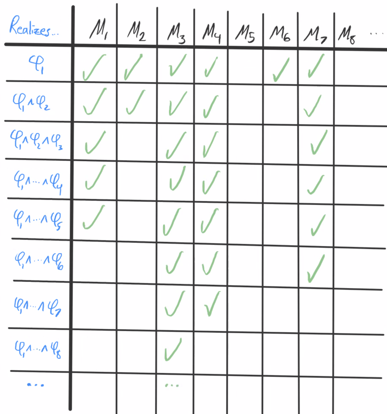
Let 𝔐 be the ultraproduct ∏(𝔐k)k∈ℕ/U. Let S = {φ1(x), φ2(x), φ3(x), …} be any countable set of formulas with countably many parameters.
Suppose S is finitely realizable in 𝔐. Then for each n, 𝔐 ⊨ ∃x (φ1(x)∧…∧φn(x)). So by Łoś’s theorem, for each n, the set of models that realize φ1(x)∧…∧φn(x) is U-large. So for each n, { k | 𝔐k ⊨ ∃x (φ1(x)∧…∧φn(x)) } ∈ U.
Here’s a visualization:
In this image, 𝔐1 realizes φ1(x)∧…∧φ5(x), 𝔐3 realizes all of S, and 𝔐5 doesn’t realize φ1(x). The finite realizability of S tells us that {1, 2, 3, 4, 6, 7, …} (the indices of models realizing φ1) is U-large. So are {1, 2, 3, 4, 7, …}, {1, 3, 4, 7, …}, {3, 4, 7, …}, and so on.
Now we add a new constant c to L. We want to define c on each 𝔐k in such a way that in 𝔐, c refers to an element of M that realizes all of S. We do this by saying that in 𝔐k, c refers to an element of Mk that realizes as large an initial segment of S as possible. More precisely:
For each finite k, consider the largest n for which 𝔐k ⊨ ∃x (φ1(x)∧…∧φn(x)). (In the above example, for k = 1 we’d have n = 5. For k = 2 we’d have n = 2. And so on.) In 𝔐k, c will refer to any object in Mk that realizes φ1 through φn. Let’s call this object ak. In other words, ak is an element of Mk that realizes as large of an initial segment of S as possible, and c refers to this element.
Two special cases: What if 𝔐k realizes all of S? Then in 𝔐k, c will refer to any ak ∈ Mk that realizes all of S. And if 𝔐k doesn’t realize φ1? Then in 𝔐k, c will refer to any arbitrary element of Mk.
One important consequence of this way of defining the “ak“s is that for any k and n, ak realizes φ1(x)∧…∧φn(x) in 𝔐k if and only if 𝔐k ⊨ ∃x (φ1(x)∧…∧φn(x)). This’ll be used in a few lines, marked by a blue =.
The ultraproduct construction now tells us exactly what c refers to in 𝔐: the equivalence class [a1, a2, a3, …]. All that’s left to do is to prove that this element of 𝔐 realizes all of S. Here’s the argument:
Let φn(x) be any arbitrary formula in S. { k | ak realizes φn in 𝔐k } ⊇ { k | ak realizes φ1(x)∧…∧φn(x) in 𝔐k } = { k | 𝔐k ⊨ ∃x (φ1(x)∧…∧φn(x)) } ∈ U. Since ultrafilters are closed under supersets, { k | ak realizes φn(x) in 𝔐k } ∈ U Since c refers to ak in 𝔐k, { k | 𝔐k ⊨ φn(c) } ∈ U. So by Łoś’s theorem, 𝔐 ⊨ φn(c). So in 𝔐, [a1, a2, a3, …] realizes φn. Since φn was an arbitrary formula in S, [a1, a2, a3, …] realizes all of S.
And we’re done! Since [a1, a2, a3, …] realizes all of S, S is realizable!
Concluding thoughts
This proof is pretty similar to the one in the last post, but with some unnecessary bells and whistles removed. Unlike the last one, this one was designed by me personally, so it’s possible there’s something important missing. But I doubt it!
It has a similar “constructive” character to the last proof, in that it doesn’t just say that S is realizable in M, it also tells you exactly what the element of M that realizes S is. I’ve noticed that this “constructiveness” is a common feature of proofs in this area of logic. Look back at our proofs of the compactness theorem. They didn’t just tell us that our starting set of sentences was satisfiable; they actually gave us a recipe for constructing a model of that set of sentences.
Now, why am I putting constructive in quotation marks? The thing is, on the traditional notion of constructiveness, none of these proofs are really constructive, because free ultrafilters can’t be shown to exist for arbitrary infinite sets without the axiom of choice. (Remember our usage of Zorn’s lemma in Part 3 of the series?) The axiom of choice is a big no-no for the constructivist, and there is a sense in which you can’t super concretely “get your hands on” a free ultrafilter. There’s no nice general procedure for specifying what’s in the ultrafilter and what’s not; if there was we wouldn’t need choice, we’d just define the ultrafilter with this procedure!
Nonetheless, I think there’s a nice notion of “conditional constructiveness”, where you say “assuming that you somehow get your hands on an ultrafilter, then what can you construct with it”. And in this sense, you can construct all the things I gave examples of earlier.
Not all nonconstructive objects are equally scary or hard-to-comprehend in my eyes, so it’s nice to be able to say something like “these are both nonconstructive in the absolute sense, but the first is constructive conditional on the existence of a free ultrafilter on the naturals, and the second is constructive conditional on the ZFC-independent existence of a large cardinal.” An approach like this frees you up to care about constructiveness without having to ascribe to the full strict Brouwerian philosophy.
I’ve spent a lot of time in the last posts gushing about how cool and powerful Łoś’s theorem is. But Łoś’s theorem is only the second most powerful property of ultraproducts that I know. The most powerful is what’s known as countable saturation.
Countable saturation is a property of structures, and it’s all about definability and parameters. Here it is in one sentence: M is countably saturated if any set of formulas using countably many parameters which is finitely realized in M is also realized in M.
Said another way, M is countably saturated means that: for any set of formulas X with countably many parameters, if the set of subsets of M defined by finite subsets of X has nonempty intersection, then there’s an object in M that satisfies all of X.
If that was a little too much to parse, don’t worry. We’ll now slowly build up to the definition by discussing definability and parameters.
Definability
Let L be some first-order language, and M be some L-structure. Suppose φ(x) is an L-formula with one free variable, x. We can consider the set of objects in the universe of M that satisfy φ: { m ∈ M | M ⊨ φ(m) }. We say that this is the set defined by φ.
For instance, let L be the language of PA and M be the natural numbers. What are the sets defined by the following formulas?
φ1(x): x > x φ2(x): x = x φ3(x): ∃y (y + y + y = x) φ4(x): ∃y (x + y = x ⋅ y) φ5(x): ∀y ∀z (y ⋅ z = x → (y = 1 ∨ z = 1))
Many many sets of naturals are definable, including uncomputable sets like the set of Busy Beaver numbers. With the language of PA, we are able to define everything on the arithmetic hierarchy, described here.
We’ll denote the set of all definable subsets of a structure M by writing D(M). So D(ℕ) is the set of all arithmetical sets.
Parameters
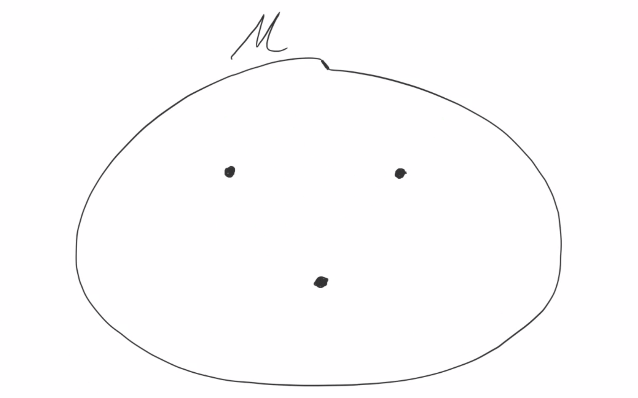
That’s definability without parameters. What about definability with parameters? Parameters are like additional constants you tack onto a language that refer to a fixed object of your choice. Let’s illustrate this with another example. Suppose that our language is empty, and our structure M contains three objects.
We don’t have any constants, so we have no way to pick out any object by name. We also don’t have any relations or functions, so we have no way to pick out any object by its properties or relationship to other objects. So take a guess, what is D(M)?
Your first thought may have been that D(M) is empty; after all if you can’t pick out any individual objects in the structure, how can you define any sets of objects? But there are still two sets of objects you can always define: the empty set (defined by any contradiction) and the entire structure (defined by any tautology).
D(M) = {∅, M}
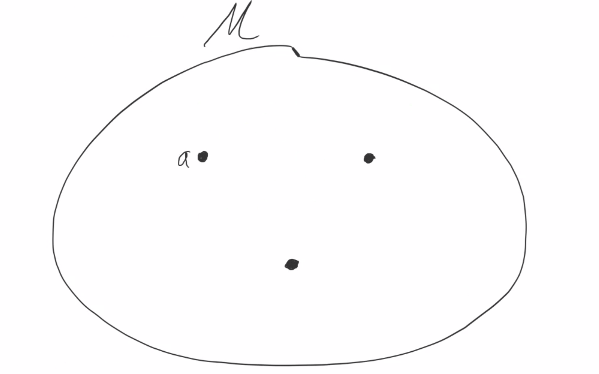
Now, suppose that we have a parameter that refers to one particular object. Let’s say the parameter is a.
We now consider formulas φ(x, a) that depend not just on the free variable x, but also this new parameter. For instance, φ(x, a): x = a. What set does this define?
We’ll write D(M, A) for the set of all subsets of M definable with parameters from A. What is D(M, {a}) in our present example?
Answer:
D(M, {a}) = {∅, {a}, M\{a}, M}
We still can’t get every subset of M, because we have no way to single out the objects besides a. Can we do it with two parameters a and b referring to distinct objects in M?
Yes! We don’t need a parameter for the third object, because we can define it with the formula “x ≠ a ∧ x ≠ b”. And once we’ve defined all singletons, we can use disjunctions to define all two-element sets. So with just two parameters, we get to define every possible subset of M.
D(M, {a,b}) = 𝒫(M)
If our structure had 4 objects instead of 3 we could do it with 3 parameters, and if it had 12 objects we could do it with 11 parameters. In general, any finite structure can be fully defined with some finite number of parameters.
Infinite structures are trickier. How many parameters are necessary to fully define ℕ in the language of PA?
Trick question! This just can’t be done in the language of PA. Adding parameters doesn’t actually let us define anything new, because every object can already be referred to: (0, S0, SS0, SSS0, …). Unlike with finite structures, having a name for every object does not guarantee that every set of objects can be defined (though it does guarantee that every finite set of objects can be defined).
But while parameters don’t help with ℕ, they do help with nonstandard models of arithmetic, as these contain objects that can’t be defined with just the symbols in the language. Suppose that K is a parameter that refers to the infinite hypernatural number [0,1,2,3,4,…]. Then { x ∈ *ℕ | x < K } is in D(*ℕ, {K}), but not in D(*ℕ, ∅). We also get { x ∈ *ℕ | x > K ∧ x is prime }, and many other sets.
Finite intersection property
We’re almost ready to define countable saturation. We just need one more concept: the finite intersection property. A set of formulas has the finite intersection property if each of its finite subsets can be realized by some object in M.
Some examples in ℕ:
(i) P = {x < 1, x < 2, x < 3, x < 4, x < 5, x < 6…} (ii) P = {x > 1, x > 2, x > 3, x > 4, x > 5, x > 6, …} (iii) P = {∃y (x = y⋅1), ∃y (x = y⋅2), ∃y (x = y⋅3), …}
For each example, we want to verify that for every finite subset of P, we can find an element that satisfies everything in that finite subset.
For instance, to show that (i) really has the finite intersection property, we think about any finite set of formulas in P, such as {x < 12, x < 33, x < 59, x < 64}. What’s an x that satisfies all of these? Obviously anything less than 12 will work, so we can take x = 11. In general, for any finite set F we can just look at the minimum n for which the sentence “x < n” appears in F and then set x = n – 1. More simply, we can just always set x = 0 and this will satisfy every finite subset.
For (ii), we can take any finite set F and find the maximum n for which the sentence x > n appears in F. Then set x = n + 1.
Figure out (iii) for yourself!
There’s an important difference you may have noticed between (i) and (ii)/(iii). Namely, in (i) we have a number (x = 0) that satisfies all of P. But in (ii) no element of c will satisfy all of P, and the same goes for (iii). (For (ii) this would correspond to an infinitely large number, and for (iii) a number that’s a multiple of every standard natural number. Notice that elements like this do exist in *ℕ!)
What this shows is that a set having the finite intersection property does not guarantee that all formulas in it can be simultaneously satisfied by a single element. That is, unless the structure in question is countably saturated!
Countable saturation
And we’ve arrived! Consider any countable set of parameters A, and then any set of formulas using these parameters. Countable saturation of M means that any such set with the finite intersection property will necessarily be satisfied by some object in M.
So for instance, if M is countably saturated, then the fact that {x is a multiple of 2, x is a multiple of 3, x is a multiple of 4, …} has the finite intersection property implies that there’s an object in M that’s a multiple of 2, 3, 4, 5, and all the rest.
Similarly, in a countably saturated model M, {x > 1, x > 2, x > 3, …} having the finite intersection property implies that there’s an object in M that’s bigger than 1, 2, 3, and every other finite number.
Clearly, ℕ isn’t countably saturated. But *ℕ is! So is *ℝ, and *ℤ! And in fact, as long as your ultraproduct is over models with a countable language and has index set ℕ, it will always be countably saturated! This is the big result we’ve been building up to.
For any countable language L and set of L-structures (M1, M2, M3, …), ∏(Mi)i∈ℕ/U is countably saturated
Let’s prove it!
The Proof
Here’s our setup:
L is a countable language (M1, M2, M3, …) is a family of L-structures U is a free ultrafilter on ℕ M = is the ultraproduct ∏(Mi)i∈ℕ/U A is a countable subset of M LA is the language L with an added constant for every a ∈ A P(x) is a countable set of LA-formulas
Suppose that P(x) is finitely realizable in M. We want to show that it’s also realizable in M. We’ll do this by explicitly constructing the element of M that realizes P(x). Since P(x) is countable, we can choose some enumeration of its formulas: P(x) = {φ1(x), φ2(x), φ3(x), …}.
Begin by writing out the sequence of all of our component models.
We’re going to now start a step-by-step process of eliminating models.
Step 1: Remove all models that don’t realize φ1.
For illustration purposes, let’s suppose that all models except M3 and M7 realize φ1.
All remaining models realize φ1.
Step 2: Remove M1, as well as all models that don’t realize φ1∧φ2.
We’ll suppose that of the remaining models, only M5 doesn’t realize φ1∧φ2. So we remove M1 and M5.
We’re now left with a set of models that all realize φ1∧φ2.
Step 3: Remove M2, as well as all models that don’t realize φ1∧φ2∧φ3.
This time we remove M6 and M10, in addition to M2.
Step 4: Remove M3, as well as all models that don’t realize φ1∧φ2∧φ3∧φ4.
M3 had already been removed, so we don’t do anything with it, but we now also remove M9.
Continue doing this process forever, so that there’s a “Step N” for every natural number N. We end up with something like this:
There’s something really important that we should notice about each of these sets of models: they’re all U-large. In other words, if at any stage we consider the set of indices of the models that remain, this set will be in U. This follows from finite realizability, by the following argument:
Suppose we consider the set of models that remain after four steps. We know that φ1∧φ2∧φ3∧φ4 is realizable in M. By Los’s theorem, this means that that the set of component models that realize φ1∧φ2∧φ3∧φ4 must be U-large. And the set of models remaining after Step 4 is exactly the set of component models that realize φ1∧φ2∧φ3∧φ4, excluding M1, M2, M3, and M4. So the remaining models form a U-large set minus a finite number of elements, which is still U-large!
Of course, the choice of “four” here was totally arbitrary. For any finite N, the set of models remaining after Step N is the set of models that realize φ1∧…∧φN (a U-large set), minus the models M1 through MN (a finite set). So these are always U-large!
Ok, we’re basically done with the proof now. All that’s left is to use our image to construct an element of M that realizes all of P(x). This construction is extremely simple! Here’s what we do:
For each model, go as many steps as you can before that model is crossed out. Visually, this is just going down each column and circling the model at the step before it is crossed out.
Look closely at the circled models. M4 is circled after Step 3, which means that it contains an element that realizes φ1∧φ2∧φ3. M8 is circled after Step 6, so it contains an element realizes φ1∧…∧φ6. And so on. For each circled model, we just pick out the element that realizes as many of the “φ”s as is promised to us by the diagram. Let’s call these elements a1, a2, a3, and so on.
Note that M3 and M7 were ruled out in Step 1. This was because they didn’t even realize φ1. These models are useless for our purposes (they aren’t able to realize any of the φs), so we just choose any arbitrary element from them. M11 wasn’t ruled out in any of the first six steps, so we can’t be sure from the diagram exactly how many of the φs it can realize. But we know that at the very latest, it’ll be removed at Step 12.
Anyway, we now have our sequence:
(a1, a2, a3, a4, …)
The equivalence class of this sequence is an element of M, and it realizes all of P(x)! Why?
Well, let’s think about which elements of the sequence (a1, a2, a3, …) realize φ1. a1 clearly does, as we chose it for that purpose. What about a2? It was chosen to realize φ1∧φ2, so of course it also realizes φ1. a3 doesn’t realize φ1, because M3 didn’t contain any element that realized φ1. a4 realizes φ1 because it realizes φ1∧φ2∧φ3∧φ4. And so on. In general, ak realizes φ1 for every k that’s the index of one of the structures in Step 1 (a U-large set!)
It might be helpful to keep in mind that when we circled a model in row k, the element we chose from that model realizes the conditions in all the earlier rows. We can visualize this as follows:
Now we can easily see which elements realize each formula:
(Bonus question: is it possible for more elements to realize φ5 than those I’ve written? Which elements? And if so, why does that not affect the proof?)
Remember how we showed that the set of models in each row was U-large? Well each of these sets of elements is U-large for the exact same reason! One more application of Łoś’s theorem and we’re done: every φ(x) in P(x) is realized by a U-large set of elements of the sequence (a1, a2, a3, …) , so every φ(x) in P(x) is realized by the element of M that is the equivalence class of this sequence: [a1, a2, a3, …].
And that’s the proof!
Hypernatural Saturation
Countable saturation is an enormously powerful tool for probing the structure of ultraproducts. Let’s see some applications.
We can use countable saturation to prove that there’s a number that’s a multiple of every finite number. We can also use it to prove that there’s a number that’s above every finite number. But we already knew all this. The real power of countable saturation shines through when we use parameters.
Take any countable set of parameters {K1, K2, K3, …}, and choose them to refer to distinct hypernaturals. Now consider the set of sentences {x is divisible by K1, x is divisible by K2, x is divisible by K3, …}. This set of sentences has the finite intersection property. Why? Because finite products always exist. Applying countable saturation, we can conclude that there’s a number that’s divisible by K1, K2, K3, and all the rest!
In other words, every countable set of hypernaturals has a multiple! This is significantly stronger than what we knew before. For one thing, it implies that there are uncountably many hypernatural primes! Suppose that there were countably many hypernatural primes. Collect them in a set P, and find a multiple N of everything in P. Now simply add 1 to N. N+1 is not divisible by any primes. It’s also larger than everything in P (use Łoś to prove this), meaning that it isn’t itself a prime. But by Łoś’s theorem, every hypernatural is either prime or composite! Contradiction.
We can also now show that *N has uncountable cofinality. In other words, every countable set of hypernaturals can be upper bounded. Let {K1, K2, K3, …} be any countable set of hypernaturals. Now consider the set of formulas {x > K1, x > K2, x > K3, …}. Every finite subset can be satisfied; simply take the largest Kn that appears in the subset and add one. Thus there’s some x that’s above the entire set {K1, K2, K3, …}. So every countable set of hypernaturals has an upper bound, meaning that any subset of *ℕ that has no upper bound must be uncountable.
We can get uncountable coinitiality of the infinite hypernaturals by a similar argument. Let {K1, K2, K3, …} be any countable set of infinite hypernaturals and consider the set of formulas {x > 0, x < K1, x > 1, x < K2, x > 2, x < K3, x > 3, …}. Fill out the rest of the argument for yourself!
Uncountable coinitiality of the infinites is a big deal! For one thing, it implies that every infinite hypernatural K is above uncountably many other hypernaturals (as otherwise the set of infinite hypernaturals below K would be a countable coinitial set of infinites). This in turn implies that distances between hypernaturals are either finite or uncountable. They cannot be countably infinite!
Why? Well, ∀x ∀y (x < y → ∃z (z + x = y)) is a sentence of TA that says essentially that for any two numbers x < y, the difference y – x exists as a number. And since we now know that all hypernaturals are either finitely large or uncountably large, we can conclude that differences must be as well!
Applying countable saturation more generally
Let L be any countable language and (Mi)i∈ℕ be any countable sequence of L-structures. We know that the ultraproduct M = ∏(Mi)i∈ℕ/U is countably saturated. Let’s further assume that M is infinite. Consider any countable set {K0, K1, K2, …} of objects in M, and apply countable saturation to the set of sentences {x ≠ K0, x ≠ K1, x ≠ K2, …} to prove that there’s some object in M outside of this set.
But the countable set {K0, K1, K2, …} was fully arbitrary! What this means is that any infinite ultraproduct M must be uncountable! We know that there are finite ultraproducts over countable languages (like the ultrapower of ℤ3, say). So any ultraproducts over a countable language with index set ℕ must be either finite or uncountable. (Exercise: where in the argument did we use the assumption that M is infinite?)
I hope that this next (and final) result blows your mind. It turns out that the continuum hypothesis (ℵ1 = 2ℵ0) has some huge implications on ultraproduct-related matters. I tend to assume that CH is false, which makes the upcoming result a little less exciting to me, but nonetheless I hope it knocks your socks off.
Continuum hypothesis and isomorphic ultrapowers
Fix some countable language L. Suppose that M1 and M2 are elementarily equivalent L-structures, and that |M1| = |M2| = ℵ0. If the continuum hypothesis is true, then the ultrapowers of M1 and M2 are isomorphic! For example, if ℕ is the standard model of arithmetic, and ℕ’ is some nonstandard countable model of true arithmetic, then *ℕ = *(ℕ’).
The proof of this is pretty nice, but to get there I need to introduce a few more notions.
So far we’ve just talked about countable saturation. But there’s a more general notion of K-saturation for any cardinal K. A structure M is K-saturated if any set of formulas using less than K parameters that’s finitely realizable in M is also realizable in M. So in a slightly annoying terminological quirk, countable saturation is actually ℵ1-saturation, as “fewer than ℵ1 parameters” is the same as “countably many parameters”.
A structure M is called saturated if it’s |M|-saturated. These structures are “as saturated as possible”. Nothing can be K-saturated for a cardinal K larger than or equal to its own size (to prove this, add a parameter for every object in the structure and declare x to differ from each of them).
Saturation is a really strong constraint on a structure. It turns out that if two structures are elementarily equivalent, the same size, and saturated, then they are necessarily isomorphic. This means that for instance there’s at most one saturated countable model of true arithmetic (up to isomorphism). The same holds for saturated models of any cardinality of Tarskian geometry, the theory of real closed fields, and any other complete theory.
And now we’re ready for the proof!
Assume that M1 and M2 are elementarily equivalent structures in a countable language, and that |M1| = |M2| = ℵ0. Take each of their ultrapowers with index set ℕ and arbitrary ultrafilters, and call them *M1 and *M2. What size are these structures? Since they’re ultraproducts, they’re both ℵ1-saturated, which means that they cannot be countable. And they’re not finite, so they must be uncountable.
Furthermore, |*M1| ≤ |M1ℕ|, as the elements of *M1 are just equivalence classes on M1ℕ. So |*M1| ≤ |M1ℕ| = ℵ0ℵ0 = 2ℵ0. Assuming the continuum hypothesis, 2ℵ0 = ℵ1. So ℵ0 < |M1| ≤ ℵ1, meaning that |*M1| = ℵ1. But remember that *M1 is ℵ1-saturated! So it’s as saturated as can be! Thus we can say that *M1 is saturated. The exact same argument goes for *M2. So *M1 and *M2 are saturated elementarily equivalent structures, and they’re both cardinality ℵ1. So they’re isomorphic!
Thus the continuum hypothesis tells us that ultrapowers erase differences between elementarily equivalent countable structures. Even though countable nonstandard models of TA look so different from the standard model, their ultraproducts are isomorphic. In particular, addition and multiplication are computable on ℕ and uncomputable on any nonstandard countable model of arithmetic. So according to CH, computable and uncomputable structures can have the same ultrapower!
We’ve seen how to use Łoś’s theorem to prove properties of hyperstructures. We’ve also seen how to use it to prove limitations of first-order logic. Today we’re going to see a major meta-logical application of Łoś’s theorem: proving the compactness theorem! In my opinion, this proof is the most elegant proof of first-order compactness out there. We’ll also see a few other meta-logical results relating to ultraproducts. However, if you’re just interested in learning about more properties of the hypernaturals, then you can skip this post without missing out on anything major!
What is compactness?
A logic is compact if any finitely satisfiable set of sentences is satisfiable. If somebody hands you an infinite set of sentences, and you know how to construct a model to satisfy any finite subset of these sentences, then you can conclude that there must be a model that satisfies all those sentences at once. Compactness is interesting because it allows you to prove surprising results (like that true arithmetic has nonstandard models) from very obvious facts (that any finite set of natural numbers has an upper bound). It also lets you prove the completeness theorem, which says that what you can prove from first-order axioms is exactly what logically follows from those axioms.
Countable Theories
First we’ll prove the compactness theorem for countable theories. I’m including it because it’s conceptually simpler than the proof of the general case. However, it’s not necessary for understanding the general proof, so if you just want to see that you can jump ahead to the next section.
Suppose T is a countably infinite theory that’s finitely satisfiable. T is countable, so choose an enumeration of T’s sentences: T = {φ1, φ2, φ3, …}.
T is finitely satisfiable, so there’s a model that satisfies φ1. Call this model M1. There’s also a model M2 that satisfies both φ1 and φ2. And a model M3 that satisfies φ1, φ2, and φ3. And so on.
Take the ultraproduct of (M1, M2, M3, …) and call it M. For every n in N, φn is satisfied by all models from Mk on. (For instance, φ4 is satisfied by M4, M5, M6, and so on.) This is a cofinite set, so (by Los’s theorem) φn is satisfied by M.
But φn was a totally arbitrary sentence inside T. So M satisfies all of T!
So T is satisfiable. But not only do we get this result, we also have an explicit example of a model that satisfies all of T, which we can start analyzing to prove other properties of.
Compactness for any theory
The proof uses a fact that I haven’t proven yet: If X is a set whose every finite subset has nonempty intersection, then there’s some ultrafilter that extends it. Luckily, it’s easily proven. Start by closing X under supersets (notice that every finite subset of X still has nonempty intersection). Then close it under intersection, and you now have a filter that extends X. (Verify that this really is a filter for bonus points!) And in Part 3 of this series we proved that every filter has an ultrafilter extension. So there’s an ultrafilter U that contains X.
Alright, on to the proof.
Let L be any first-order language and S be any set of L-sentences that is finitely satisfiable. We’re going to build an ultraproduct that satisfies S. This requires three ingredients: an index set I, and a set of L-structures (Mi)i∈I indexed by I, and an ultrafilter U on I. We’ll go through these one at a time.
1. The index set I
I will be the set of all finite subsets of S. This is interestingly different from what we’ve seen before. Previously our indices were always natural numbers. But here our indices are sets of sentences in the language of the structure! This means that we’re going to end up looking at models that look like M{φ,ψ,θ}, where φ,ψ, and θ are sentences in S.
2. The component structures (Mi)i∈I
So, our indices are finite subsets of S. And S is finitely satisfiable. So for each index F (each finite subset of S), there’s a model MF that satisfies everything in F. This is how we get our component structures.
For instance, if φ, ψ, and θ are three sentences in S, then {φ,ψ,θ} is an index, and M{φ,ψ,θ} is any structure that satisfies φ∧ψ∧θ. ∅ is also a finite subset of S, so it’s an index and has a corresponding structure M∅, which can be any L-structure whatsoever.
To briefly rehash, the important feature of our choice of component structures is that they have the following property: For any finite subset F of S, MF ⊨ φ for every φ in F.
3. The ultrafilter U on I
The choice of ultrafilter here is really important. Our component structures were carefully chosen so that each structure satisfies the finite set of sentences that is its index. This guarantees us that for any sentence φ in S, the set of component structures whose indices contain φ all satisfy φ. This is the set of component structures whose indices are finite supersets of {φ}.
Remember that we’re ultimately aiming to show that each φ is satisfied by the ultraproduct model. By Łoś’s theorem, it suffices to show that the set of component models that satisfy φ is U-large (is in our chosen ultrafilter). Conclusion: we want to make sure that for any φ in S, the set of all finite supersets of {φ} is U-large.
How do we know that there exists any ultrafilter that for every φ contains the set of all finite supersets of {φ}? We apply the finite intersection property! Denote by SF the set of all finite supersets of F. Take any finite set of singletons {{φ1}, {φ2}, {φ3}, …, {φn}}. Is the intersection of S{φ1}, S{φ2}, S{φ3}, …, S{φn} empty? No: the set {φ1, φ2, φ3, …, φn} is in of all of them! So the set { S{φ} | φ ∈ S } has the finite intersection property, and thus there’s some ultrafilter that extends it. And that’s the ultrafilter we want!
Finalizing things
We’ve now got everything we need to build the structure that satisfies S. Take the ultraproduct Π(MF)F∈I/U. This structure satisfies S. Why?
Consider any φ in S. By Łoś’s theorem, φ is satisfied if a U-large set of the component models satisfy φ. And we know that a U-large set of component models satisfy φ, because φ is satisfied in every model whose index contains φ, i.e. the set of models whose indices are supersets of {φ}. So we’re done!
More implications
The remainder of this post will not be necessary to understand the rest of the series. I want to present a few miscellaneous meta-logical results that relate to ultraproducts that don’t quite fit anywhere else.
First: every finite structure is its own ultrapower. Let’s see why.
Suppose M is a finite structure. Denote by MI/U the ultrapower of M over any arbitrary index set I. First of all, we can easily see that M and MI/U have the same cardinality: if |M| = n for some finite n, then there’s a sentence affirmed by M that says “There are exactly n distinct things”. For instance, if M has exactly two elements, then M ⊨ ∃x ∃y (x≠y ∧ ∀z (z=x ∨ z=y)). Łoś tells us that MI/U also affirms this sentence, so MI/U also has exactly n distinct things.
Furthermore, any finite structure M of size n can be categorically specified up to isomorphism by a single first-order sentence of the form ∃x1∃x2…∃xn (∀x (x = x1 ∨ … ∨ x = xn) ∧ (x1 ≠ x2 ∧ … xn-1 ≠ xn) ∧ ψ(x1, …, xn) ], where ψ specifies the behavior of all relation, function, and constant symbols. Here’s an example for a simple finite structure:
We have four elements, so we use four variables, x1 x2 x3 and x4 to specify the structure.
Since M satisfies this sentence, Łoś tells us that MI/U also affirms this sentence, meaning that MI/U and M are isomorphic. So in other words, every finite structure is its own ultrapower (up to isomorphism).
What about infinite structures? The situation is the exact opposite! No infinite structure is its own ultrapower.
Let M be an infinite structure and *M be its ultrapower. Add a constant for every object in M. The ultraproduct construction tells you how constants from M translate to constants in *M: for each constant c, if c refers to m in M, then c refers to [m, m, m, …] in *M.
Now we want to construct a new element of *M by writing a sequence that contains infinitely many elements of M, each appearing only finitely many times. Crucially, here we must assume that the index set is the same size as or smaller than M! If we have too many indices, then we aren’t going to be able to refer to each element in our original model only a finite number of times. So for instance, this argument won’t work for the ultrapower ℕℝ/U.
Now, this new element we’ve constructed is distinct from each constant, because they only agree in finitely many place. The constants covered all of M, but they don’t cover all of *M. So M and *M are not isomorphic!
And some more
These next results relate ultraproducts to compactness and definability.
Fix a first-order language L and consider a class C of L-structures. Say that a set of sentences X is C-satisfiable if there’s a structure in C that satisfies all of X. We say that C is compact if for every set A of L-formulas, finite C-satisfiability implies C-satisfiability. This is a different notion from the compactness discussed in the compactness theorem; the ordinary compactness theorem tells us that for every first-order language L, the class of all L-structures is compact. But it doesn’t tell us anything about other more restricted classes of L-structures.
For instance, let L be the language with an empty signature (no constants, functions or relations). This language is extremely simple: essentially the only contentful sentences you can make are about finite cardinalities. E.g. you can say “there are at least three things” with “∃x ∃y ∃z (x≠y ∧ x≠z ∧ y≠z)” and “there are at most three things” with “∀x ∀y ∀z ∀w (x=y ∨ x=z ∨ x=w ∨ y=z ∨ y=w ∨ z=w)”.
Now let C be the class of all finite L-structures. Is this class compact?
If you said no, good job! For a finite n, let φn be the sentence that says “there are at least n things”, and consider the set of sentences A = {φ1, φ2, φ3, …}. Every finite subset of A is satisfiable by a finite L-structure, but the entire set is clearly not satisfiable by any finite L-structure.
What if we add to C a single countably infinite L-structure M? Then our previous construction no longer works; the entire set A is now satisfied by this new member of C.
Alright, so that’s compactness for classes of structures. The relationship between this and ultraproducts is the following:
Any class of models that’s closed under ultraproducts is also compact.
For any language L and any finite n, consider the class of all L-structures of size n. The ultraproduct of a bunch of size-n L-structures is itself a size-n L-structure, so this class is closed under ultraproducts. And therefore it’s compact!
Now consider our example of the class of all finite structures in the language with empty signature. This was not compact, meaning that it cannot be closed under ultraproducts. This means that the ultraproduct of a bunch of finite structures is not necessarily finite! In particular, suppose that M1 has one element, M2 has two elements, M3 has three elements, and so on. Then the ultraproduct of (M1, M2, M3, …) will be an infinite model. We can also see this by applying Łoś’s theorem to the set of sentences {“There is at least 1 thing.”, “There are at least 2 things.”, “There are at least 3 things.”, …}.
A class C of L-structures is first-order definable if it is the set of all models of some set of L-sentences. First-order definability also relates to ultraproducts, in the following way:
If a class of L-structures is first-order definable, then it’s closed under ultraproducts.
The converse of this is that any class of structures that’s not closed under ultraproducts is not definable.
For any L, the class of finite L-structures is not closed under ultraproducts, so it’s not definable. This tells us that “finiteness” is not first-order definable.
The class of all models of PA is first-order definable, so it’s closed under ultraproducts. This means that even if you take an ultraproduct of infinitely many nonstandard models of PA, you still end up with a model of PA!
Okay, next up we come to the most exciting and powerful property of ultraproducts: countable saturation!
The hypernaturals, *ℕ, are the ultrapower of ℕ with index set I = ℕ. The first-order language in use here is the language of Peano arithmetic: L = <{0}, {<}, {S,+,⋅}>. Łoś’s theorem from the last post tells us that *ℕ and ℕ are elementarily equivalent. In other words:
For every first-order sentence φ, ℕ ⊨ φ if and only if *ℕ ⊨ φ.
This tells us that *ℕ is not just a model of Peano arithmetic, which is a popular incomplete theory of arithmetic. It’s a model of TRUE arithmetic, the complete set of all first-order truths of arithmetic! Given the insane uncomputability of this theory (If T0 is a Turing machine, and Tn+1 is a Turing machine with an oracle for Tn‘s halting problem, then true arithmetic is not computable by Tn for any finite n), it’s pretty remarkable that we have an explicit example of one of its nonstandard models!
Review over! Now let’s begin with some basic applications of Łoś’s theorem. We can say that a number x is prime in first-order logic: isPrime(x) can be translated as ∀y ∀z (y⋅z = x → (y = 1 ∨ z = 1)). We can also refer to any finite natural number by applying the successor function enough times to zero (e.g. 2 = S(S(0))). Since “2 is a prime” is first-order expressible and ℕ affirms its truth, so must *ℕ.
But remember that in *ℕ, 2 is the equivalence class of the sequence (2,2,2,2,…). Is it really true that for any a, b ∈ *ℕ, if a⋅b = [2,2,2,2,…] then one of a and b is 2 and the other is 1? This is probably not immediately obvious… What about (2,1,2,1,2,1,…)⋅(1,2,1,2,1,2,…)? Certainly this product is (2,2,2,2,…), but neither (2,1,2,1,2,1,…) nor (1,2,1,2,1,2,…) look very much like (1,1,1,1,…) or (2,2,2,2,…).
In fact they are the same. Let’s prove this very generally. Suppose p is any finite prime number, and consider the hypernatural [p, p, p, …], corresponding to the ordinary natural number p. Consider any two hypernaturals a and b such that a⋅b = p. We can choose representative sequences (a0, a1, a2, …) and (b0, b1, b2, …) such that their product is (p, p, p, …). In other words:
(a0⋅b0, a1⋅b1, a2⋅b2, …) = (p, p, p, …)
Since p is prime, we know that for each k, either (ak = p and bk = 1) or (ak = 1 and bk = p). Consider the set of indices A = { k ∈ ℕ | ak = p }. Since each ak is either 1 or p, the complement ℕ\A is equal to { k ∈ ℕ | ak = 1 }. Now, since U is an ultrafilter, either A or ℕ\A is in U. In the first case, [a0, a1, a2, …] = [p, p, p, …] = p. And in the second case, [a0, a1, a2, …] = [1, 1, 1, …] = 1. The same argument applies for [b0, b1, b2, …]. So for any two hypernaturals a and b such that a⋅b = p, both a and b are either 1 or p.
Okay, so we’ve proven that 2 is a prime number. That’s a relief! Let’s do something a bit more substantial now.
Consider the following first-order sentence: ∀x ∃y (y > x ∧ isPrime(y)). This sentence says that there are infinitely many primes, and (as first proven by Euclid) ℕ affirms its truth. So *ℕ ⊨ ∀x ∃y (y > x ∧ isPrime(y)).
Okay, so there are infinitely many hypernatural primes. This doesn’t sound so exciting… after all every ordinary prime is a hypernatural prime too, so didn’t we already know this? Sure, but if we look closely at what exactly the sentence says, it turns out that we get a bit more out of it than just that.
∀x ∃y (y > x ∧ isPrime(y)) says that for every number x, there’s a larger prime number y. Applying this in *ℕ, this means that all hypernatural numbers, even the infinitely large ones, have larger primes. Thus there are nonstandard primes in *ℕ, and in fact infinitely many nonstandard primes.
See if you can think of one for yourself before reading on.
.
.
.
Ok, here’s one: P = [2, 3, 5, 7, 11, 13, 17, …]. This sequence is eventually always larger than the sequence of any standard prime p = [p, p, p, p, …], so P is a nonstandard number. And P is also prime! The argument is very similar to the previous argument: take any two hypernaturals a and b such that a⋅b = k. Consider any representative sequences for a and b whose product is the sequence (2, 3, 5, 7, 11, …), and then consider the set of indices at which 1 appears in a’s sequence. If this set is in the ultrafilter, then a = 1 and b = k. If not, then a = k and b = 1.
Now, a challenge for you: construct an infinite ascending sequence of nonstandard primes starting at P.
And another challenge: construct an infinite descending sequence of nonstandard primes starting at P!
Hint for the first challenge: think about the hypernatural [3, 5, 7, 11, 13, 17, …].
Hint for the second challenge: think about the hypernatural [2, 2, 3, 5, 7, 11, …], or [2, 2, 3, 3, 5, 5, 7, 7, …].
While infinite ascending sequences of numbers can exist in ℕ, an infinite descending sequence of numbers can not, so we’ve identified a concrete difference between *ℕ and ℕ. And by Łoś’s theorem, this difference must not be first-order expressible in the language of PA. In other words, “there are no infinitely descending sequences of numbers” cannot be expressed in first-order.
This illustrates another usage of Łoś’s theorem: rather than starting with a first-order sentence that’s true of ℕ and using it to learn about *ℕ, we can start with some facts about *ℕ to learn about limitations of first-order logic!
Alright, what else? Suppose we have a hypernatural number k that has a sequence (k0, k1, k2, …) such that some formula φ(x) holds of cofinitely many elements of the sequence. Then φ(x) also holds of k. This gives us some hypernatural numbers with awfully strange properties.
Consider the hypernatural E = [1, 2, 4, 8, 16, 32, 64, …]. Now consider the formulas that say “x is divisible by 2”, “x is divisible by 4”, “x is divisible by 8”, “x is divisible by 16”, and so on. Each of these formulas holds true of all but some initial segment of the sequence (1, 2, 4, 8, 16, 32, 64, …). This means that each of these sentences hold true of E. In other words, E is divisible by 2, by 4, by 8, by 16, by 32, and so on forever. In other words, E can be divided by 2 forever!
But how exactly does this work? The sequence (1, 2, 4, 8, 16, 32, 64, …) starts with a 1. So how could we divide it by 2? The key is to remember that hypernaturals are equivalence classes of sequences, not sequences. So any time we run into trouble with a particular sequence, we can jump to an equivalent sequence that solves our problem. To divide (1, 2, 4, 8, 16, 32, 64, …) by 2, we jump to the equivalent sequence (2, 2, 4, 8, 16, 32, 64, …), which is still a representative of E. Now we can divide by 2: E/2 = [1, 1, 2, 4, 8, 16, 32, …]. To divide by 2 again, we jump to the sequence (2, 2, 2, 4, 8, 16, 32, …). Then we get E/4 = [1, 1, 1, 2, 4, 8, 16, …]. We can keep doing this as many times as we like, and thus E is infinitely even! (Notice: another infinitely descending sequence of numbers.)
We can use a similar trick to construct a number that’s divisible by every standard natural number: simply consider M = [0!, 1!, 2!, 3!, 4!, 5!, …]. For any standard natural number n, the set of indices at which the sequence (0!, 1!, 2!, 3!, 4!, 5!, …) can be divided by n is cofinite. So M can be divided by n as well!
This lets us run a kind of fun argument. Remember how Euclid’s original proof of the infinitude of primes went? Imagine that there are finitely many primes. Then we can take their product and add 1, and we’ve constructed a new prime. Well, in *ℕ we can find multiples of infinite sets of numbers! One multiple of all standard prime numbers is [2, 2⋅3, 2⋅3⋅5, 2⋅3⋅5⋅7, 2⋅3⋅5⋅7⋅11, …] = [2, 6, 30, 210, 2310, …]. This is divisible by each standard prime, and is also not twice-divisible by any prime (e.g. you can’t divide it by 4). (Interestingly, it’s not the product of all finite primes; because it’s also divisible by some infinite primes! See if you can think of one such infinite factor.) Now add 1 to get X = [3, 7, 31, 211, 2311, …]. X cannot be divisible by any standard prime, meaning that it’s either divisible by a nonstandard prime, or is itself a nonstandard prime. So just as Euclid’s original proof showed that there can’t be only finitely many primes, this proves that there can’t be only finitely large primes.
Alright, let’s get a little more wild. In ℕ we know that for any number x, there’s a number y that’s divisible by all positive numbers up to and including x (for instance, y = x!). In other words, ℕ ⊨ ∀x ∃y ∀z ((z ≠ 0 ∧ z ≤ x) → (y div by z)), where “y div by z” is shorthand for ∃u (z⋅u = y). In other words, ℕ affirms that for every initial segment S with maximum element x, there’s a number that’s divisible by everything in S (for shorthand we can call this number “a multiple of S”).
Invoke Łoś: anything true in ℕ must also be true in *ℕ. This means that every initial segment of hypernaturals with a maximum element has a multiple! (See if you can do better: can you also prove that every initial segment of hypernaturals with a max has a product? What about initial segments without maximum elements?) For instance, there’s a number that’s divisible by every hypernatural number up to and including the hypernatural K = [0,1,2,3,4,5,…].
What other first-order properties does ℕ have? Here’s one: ℕ is not dense. We can express this by saying ¬(∀x ∀z (x < z → ∃y (x < y ∧ y < z)). We can do better: ℕ affirms that ∀x ¬∃y (x < y ∧ y < S(x)). In other words, for any number x, x and its successor are counterexamples to density (they’re distinct numbers that have nothing between them).
So this must be true of hypernaturals as well! For any hypernatural, say K = [0,1,2,3,4,5,…], there’s no hypernatural between it and its successor K+1 = [1,2,3,4,5,6,…].
However, even though the hypernaturals are not dense, they do contain a dense subset! In fact, we can say something even stronger: no segment of the hypernaturals are dense, but nonetheless *ℕ has a dense subset!
Here’s a rough sketch for how to construct this dense subset. Take any nonstandard hypernatural, say K = [0, 1, 2, 3, 4, 5, …]. For any nonzero finite m, we can construct a hypernatural Km a finite distance from K, such that K’ is divisible by m. Now we can construct n⋅Km, and then (n/m)⋅Km. The set { (n/m)⋅Km | n, m ∈ ℕ } is a subset of the hypernaturals, and it has the order type of the positive rationals!
What other unusual hypernatural numbers can you discover?
Next, we will prove the compactness theorem using ultraproducts. It’s definitely the prettiest proof of compactness out there, so stay tuned!