Will we ever build a Galactic Empire?

December 27, 2019 ~ squarishbracket ~ Leave a comment

I devoured science fiction as a kid. One of my favorite books was Asimov’s Foundation, which told the story of a splintering Galactic Empire and the seeds of a new civilization that would grow from its ashes. I marveled and was filled with joy at the notion that in our far future humanity might spread across the galaxy, settling countless new planets and bringing civilization to every corner of it.

Then I went to college and learned physics, especially special relativity and cosmology, and learned that there are actually some hugely significant barriers in the way of these visions ever being manifest in reality. Ever since, it has seemed obvious to me that the idea of a galactic civilization, or of humans “colonizing the universe” are purely fantasy. But I am continuously surprised when I hear those interested in futurism throw around these terms casually, as if their occurrence were an inevitability so long as humans stay around long enough. This is deeply puzzling to me. Perhaps these people are just being loose with their language, and when they refer to a galactic civilization, they mean something much more modest, like a loosely-connected civilization spread across a few nearby stars. Or maybe there is a fundamental misunderstanding of both the limitations imposed on us by physics and the the enormity of the scales in question. Either way, I want to write a post explaining exactly why these science fiction ideas are almost certainly never going to become reality.

My argument in brief:

We are really slow.
The galaxy is really big.
The universe is even bigger.

Back in 1977, humans launched the Voyager 1 spacecraft, designed to explore the outer solar system and then to head for the stars. Its trajectory was coordinated to slingshot around Jupiter and then Saturn, picking up speed at each stage, and then finally to launch itself out of the solar system into the great beyond. 36 years later, in 2012, it has finally left the Sun’s heliopause, marking the first steps into interstellar space. It is now 11.7 billion miles from Earth, which sounds great until you realize that this distance is still less than two-tenths of a single percent of one light year.

Compare this to, say, the distance to the nearest star Alpha Centauri, we find that it has traveled less than .05% of the distance. At this rate, it would take another 80,000 years to make contact with Alpha Centauri (if it were aimed in that direction)! On the scale of distances between stars, our furthest current exploration has gotten virtually nowhere. It’s the equivalent of somebody who started in the center of the Earth hoping to burrow up all the way to the surface, and takes 5 days to travel a single meter. Over 42 years, they would have travelled just under 3000 meters.

OK, you say, but that’s unfair. The Voyager was designed in the 70s! Surely we could do better with modern space shuttle design. To which my reply is, sure we can do better now, but not better enough. The fastest thing humans have ever designed is the Helios 2 shuttle, which hit a speed of 157,078 mph at its fastest (.023% of the speed of light). If we packed some people in this shuttle (which we couldn’t) and sent it off towards the nearest star (assuming that it stayed at this max speed the entire journey), guess how long it would take? Over 18 thousand years.

And keep in mind, this is only talking about the nearest star, let alone spreading across the galaxy! It should be totally evident to everybody that the technology we would need to be able to reach the stars is still far far away. But let’s put aside the limits of our current technology. We are still in our infancy as a space-faring species in many ways, and it is totally unfair to treat our current technology level as if it’s something set in stone. Let’s give the futurists the full benefit of the doubt, and imagine that in the future humans will be able to harness incredible quantities of energy that vastly surpass anything we have today. If we keep increasing our energy capacity more and more, is there any limitation on how fast we could get a spacecraft going? Well, yes there is! There is a fundamental cosmic speed limit built into the of the universe, which is of course the speed of light. The speed-vs-energy curve has a vertical asymptote at this value; no finite amount of energy can get you past this speed.

So much for arbitrarily high speeds. What can we do with spacecraft traveling near the speed of light? It turns out, a whole lot more! Suppose we can travel at 0.9 times the speed of light, and grant also that the time to accelerate up to this speed is insignificant. Now it only takes us 4.7 years to get to the nearest star! The next closest star takes us 6.6 years. Next is 12.3 years. This is not too bad! Humans in the past have made years-long journeys to discover new lands. Surely we could do it again to settle the stars.

But now let’s consider the trip to the center of the galaxy. At 90% the speed of light, this journey would take 29,000 years. As you can see, there’s a massive difference between jumping to nearby stars and attempting to actually traverse the galaxy. The trouble is that most people don’t realize just how significant this change in distance scale is. When you hear “distance to Alpha Centauri” and “distance to the center of the Milky Way”, you are probably not intuitively grasping how hugely different these two quantities are. Even if we had a shuttle traveling at 99.99% times the speed of light, it would take over 100,000 years to travel the diameter of the Milky Way.

You might be thinking “Ok, that is quite a long time. But so what! Surely there will be some intrepid explorers that are willing to leave behind the safety of settled planets to bring civilization to brand new worlds. After all, taking into account time dilation, a 1000 year journey from Earth’s perspective only takes 14 years to pass from the perspective of a passenger on a ship traveling at 99.99% percent of the speed of light.”

And I accept that! It doesn’t seem crazy that if humans develop shuttle that travel a significant percentage of the speed of light, we could end up with human cities scattered all across the galaxy. But now the issue is with the idea of a galactic CIVILIZATION. Any such civilization faces a massive problem, which is the issue of communication. Even having a shared society between Earth and a planet around our nearest star would be enormously tricky, being that any information sent from one planet to the other would take more than four years to arrive. The two societies would be perpetually four years behind each other, and this raises some serious issues for any central state attempting to govern both. And it’s safe to say that no trade can exist between two planets that have a 10,000 year delay in communication. Nor can any diplomacy, or common leadership, or shared culture or technology, or ANY of the necessary prerequisites for a civilization.

I think that for these reasons, it’s evident that the idea of a Galactic Empire like Asimov’s could never come into being. The idea of such a widespread civilization must rely on an assumption that humans will at some point learn to send faster than light messages. Which, sure, we can’t rule out! But everything in physics teaches us that we should be betting very heavily against it. Our attitude towards the idea of an eventual real life Galactic Empire should be similar to our attitude towards perpetual motion machines, as both rely on a total rewriting of the laws of physics as we know them.

But people don’t stop at a Galactic Empire. Not naming names, but I hear people that I respect throwing around the idea that humans can settle the universe. This is total madness. The jump in distance scale from diameters of galaxies to the size of the observable universe, is 40 times larger than the jump in distance scale we previously saw from nearby stars to galactic diameters. The universe is really really big, and as it expands, every second more of it is vanishing from our horizon of observable events.

Ok, so let’s take the claim to be something much more modest than the literal ‘settle galaxies all across the observable universe’. Let’s take it that they just mean that humans will spread across our nearest neighborhood of galaxies. The problem with this is again that the distance scale in question is just unimaginably large. Clearly we can’t have a civilization across galaxies (as we can’t even have a civilization across a single galaxy). But now even making the trip is a seemingly insurmountable hurdle. The Andromeda Galaxy (the nearest spiral galaxy to the Milky Way) is 2 million light years away. Even traveling at 99.99% of the speed of light, this would be a 28,000 year journey for those within the ship. From one edge of the Virgo supercluster (our cluster of neighbor galaxies) to the other takes 110 million years at the speed of light. To make this trip doable in a single lifetime requires a speed of 99.999999999999% of c (which would result in the trip taking 16 years inside the spacecraft). The kinetic energy required to get a mass m to these speeds is given by KE = (γ – 1) mc². If our shuttle and all the people on it have a mass of, say, 1000 kg, the required energy ends up being approximately the entire energy output of the Sun per second.

Again, it’s possible that if humans survive long enough and somehow get our hands on the truly enormous amounts of energy required to get this close to the speed of light, then we could eventually have human societies springing up in nearby galaxies, in total isolation from one another. But (1) it’s far from obvious that we will ever be capable of mastering such enormous amounts of energy, and (2) I think that this is not what futurists are visualizing when they talk about settling the universe.

Let me just say that I still love science fiction, love futurism, and stand in awe when I think of all the incredible things the march of technological progress will likely bring us in the future. But this seems to be one area where the way that our future prospects are discussed is really far off the mark, and where many people would do well to significantly adjust their estimates of the plausibility of the future trajectories they are imagining. Though science and future technology may bring us many incredible new abilities and accomplishments as a species, a galactic or intergalactic civilization is almost certainly not one of them.

Solving the Linear Cournot Model

December 2, 2019December 2, 2019 ~ squarishbracket ~ 3 Comments

The Cournot model is a simple economic model used to describe what happens when multiple companies compete with one another to produce some homogenous product. I’ve been playing with it a bit and ended up solving the general linear case. I assume that this solution is already known by somebody, but couldn’t find it anywhere. So I will post it here! It gives some interesting insight into the way that less-than-perfectly-competitive markets operate. First let’s talk about the general structure of the Cournot model.

Suppose we have n firms. Each produces some quantity of the product, which we’ll label as $q_1, q_2, ..., q_n$ . The total amount of product on the market will be given the label $Q = q_1 + q_2 + ... + q_n$ . Since the firms are all selling identical products, it makes sense to assume that the consumer demand function $P(q_1, q_2, ..., q_n)$ will just be a function of the total quantity of the product that is on the market: $P(q_1, q_2, ..., q_n) = P(q_1 + q_2 + ... + q_n) = P(Q)$ . (This means that we’re also disregarding effects like customer loyalty to a particular company or geographic closeness to one company location over another. Essentially, the only factor in a consumer’s choice of which company to go to is the price at which that company is selling the product.)

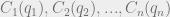
For each firm, there is some cost to producing the good. We capture this by giving each firm a cost function $C_1(q_1), C_2(q_2), ..., C_n(q_n)$ . Now we can figure out the profit of each firm for a given set of output values $q_1, q_2, ..., q_n$ . We’ll label the profit of the kth firm as $\Pi_k$ . This profit is just the amount of money they get by selling the product minus the cost of producing the product: $\Pi_k = q_k P(Q) - C_k(q_k)$ .

If we now assume that all firms are maximizing profit, we can find the outputs of each firm by taking the derivative of the profit and setting it to zero. $\frac{d\Pi_k}{dq_k} = P(Q) + q_k \frac{dP}{dQ} - \frac{dC_k}{dq_k} = 0$ . This is a set of n equations with n unknown, so solving this will fully specify the behavior of all firms!

Of course, without any more assumptions about the functions $P$ and $C_k$ , we can’t go too much further with solving this equation in general. To get some interesting general results, we’ll consider a very simple set of assumptions. Our assumptions will be that both consumer demand and producer costs are linear. This is the linear Cournot model, as opposed to the more general Cournot model.

In the linear Cournot model, we write that $P(Q) = a - bQ$ (for some a and b) and $C_k(q_k) = c_k q_k$ . As an example, we might have that P(Q) = $100 – $2 × Q, which would mean that at a price of $40, 30 units of the good will be bought total.

demand curve.png

The constants $c_k$ represent the marginal cost of production for each firm, and the linearity of the cost function means that the cost of producing the next unit is always the same, regardless of how many have been produced before. (This is unrealistic, as generally it’s cheaper per unit to produce large quantities of a good than to produce small quantities.)

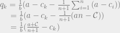
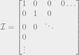
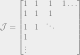
Now we can write out the profit-maximization equations for the linear Cournot model. $\frac{d\Pi_k}{dq_k} = P(Q) + q_k \frac{dP}{dQ} - \frac{dC_k}{dq_k} = a - bQ - b q_k - c_k = 0$ . Rewriting, we get $q_k + Q = \frac{a - c_k}{b}$ . We can’t immediately solve this for $q_k$ , because remember that Q is the sum of all the quantities produced. All n of the quantities we’re trying to solve are in each equation, so to solve the system of equations we have to do some linear algebra!

$2q_1 + q_2 + q_3 + ... + q_n = \frac{a - c_1}{b} \\ q_1 + 2q_2 + q_3 + ... + q_n = \frac{a - c_2}{b} \\ q_1 + q_2 + 2q_3 + ... + q_n = \frac{a - c_2}{b} \\ \ldots \\ q_1 + q_2 + q_3 +... + 2q_n = \frac{a - c_n}{b}$

Translating this to a matrix equation…

$\begin{bmatrix} 2 & 1 & 1 & 1 & 1 & \ldots \\ 1 & 2 & 1 & 1 \\ 1 & 1 & 2 & & \ddots \\ 1 & 1 & & \ddots \\ 1 & & \ddots \\ \vdots \end{bmatrix} \begin{bmatrix} q_1 \\ q_2 \\ q_3 \\ \vdots \\ q_{n-2} \\ q_{n-1} \\ q_n \end{bmatrix} = \frac{1}{b} \begin{bmatrix} a - c_1 \\ a - c_2 \\ a - c_3 \\ \vdots \\ a - c_{n-2} \\ a - c_{n-1} \\ a - c_n \end{bmatrix}$

Now if we could only find the inverse of the first matrix, we’d have our solution!

$\begin{bmatrix} q_1 \\ q_2 \\ q_3 \\ \vdots \\ q_{n-2} \\ q_{n-1} \\ q_n \end{bmatrix} = \begin{bmatrix} 2 & 1 & 1 & 1 & 1 & \ldots \\ 1 & 2 & 1 & 1 \\ 1 & 1 & 2 & & \ddots \\ 1 & 1 & & \ddots \\ 1 & & \ddots \\ \vdots \end{bmatrix} ^{-1} \frac{1}{b} \begin{bmatrix} a - c_1 \\ a - c_2 \\ a - c_3 \\ \vdots \\ a - c_{n-2} \\ a - c_{n-1} \\ a - c_n \end{bmatrix}$

I found the inverse of this matrix by using the symmetry in the matrix to decompose it into two matrices that were each easier to work with:

$\mathcal{I} = \begin{bmatrix} 1 & 0 & 0 & 0 \ldots \\ 0 & 1 & 0 \\ 0 & 0 & \ddots \\ 0 \\ \vdots \end{bmatrix}$

$\mathcal{J} = \begin{bmatrix} 1 & 1 & 1 & 1 \ldots \\ 1 & 1 & 1 \\ 1 & 1 & \ddots \\ 1 \\ \vdots \end{bmatrix}$

$\begin{bmatrix} 2 & 1 & 1 & 1 & 1 & \ldots \\ 1 & 2 & 1 & 1 \\ 1 & 1 & 2 & & \ddots \\ 1 & 1 & & \ddots \\ 1 & & \ddots \\ \vdots \end{bmatrix} = \mathcal{I} + \mathcal{J}$

As a hypothesis, suppose that the inverse matrix has a similar form (one value for the diagonal elements, and another value for all off-diagonal elements). This allows us to write an equation for the inverse matrix:

$(\mathcal{I} + \mathcal{J}) (A \mathcal{I} + B \mathcal{J}) = \mathcal{I}$

To solve this, we’ll use the following easily proven identities.

$\mathcal{I} \cdot \mathcal{I} = \mathcal{I} \\ \mathcal{I} \cdot \mathcal{J} = \mathcal{J} \\ \mathcal{J} \cdot \mathcal{I} = \mathcal{J} \\ \mathcal{J} \cdot \mathcal{J} = n \mathcal{J} \\$

$(\mathcal{I} + \mathcal{J}) (A \mathcal{I} + B \mathcal{J}) \\ = A \mathcal{I} + A \mathcal{J} + B \mathcal{J} + nB \mathcal{J} \\ = A \mathcal{I} + \left( A + B(n+1) \right) \mathcal{J} \\ = \mathcal{I}$

$A = 1 \\ A + B(n+1) = 0$

$A = 1 \\ B = - \frac{1}{n+1}$

$(\mathcal{I} + \mathcal{J})^{-1} = \mathcal{I} - \frac{1}{n+1} \mathcal{J} = \frac{1}{n+1} \begin{bmatrix} n & -1 & -1 & -1 & -1 & \ldots \\ -1 & n & -1 & -1 \\ -1 & -1 & n & & \ddots \\ -1 & -1 & & \ddots \\ -1 & & \ddots \\ \vdots \end{bmatrix}$

Alright awesome! Our hypothesis turned out to be true! (And it would have even if the entries in our matrix hadn’t been 1s and 2s. This is a really cool general method to find inverses of this family of matrices.) Now we just use this inverse matrix to solve for the output from each firm!

$\begin{bmatrix} q_1 \\ q_2 \\ q_3 \\ \vdots \\ q_{n-2} \\ q_{n-1} \\ q_n \end{bmatrix} = (\mathcal{I} - \frac{1}{n+1} \mathcal{J}) \ \frac{1}{b} \begin{bmatrix} a - c_1 \\ a - c_2 \\ a - c_3 \\ \vdots \\ a - c_{n-2} \\ a - c_{n-1} \\ a - c_n \end{bmatrix}$

Define: $\mathcal{C} = \sum_{i=1}^{n}{c_i}$

$q_k = \frac{1}{b} (a - c_k - \frac{1}{n+1} \sum_{i=1}^{n}{(a - c_i)}) \\ ~~~~ = \frac{1}{b} (a - c_k - \frac{1}{n+1} (an - \mathcal{C})) \\ ~~~~ = \frac{1}{b} (\frac{a + \mathcal{C}}{n+1} - c_k)$

$Q^* = \sum_{k=1}^n {q_k} \\ ~~~~~ = \frac{1}{b} \sum_{k=1}^n ( \frac{a + \mathcal{C}}{n+1} - c_k ) \\ ~~~~~ = \frac{1}{b} \left( \frac{n}{n+1} (a + \mathcal{C}) - \mathcal{C} \right) \\ ~~~~~ = \frac{1}{b} \left( \frac{n}{n+1} a - \frac{\mathcal{C}}{n+1} \right) \\ ~~~~~ = \frac {an - \mathcal{C}} {b(n+1)}$

$P^* = a - bQ^* \\ ~~~~~ = a - \frac{an - \mathcal{C}}{n+1} \\ ~~~~~ = \frac{a + \mathcal{C}}{n+1}$

$\Pi_k^* = q_k^* P^* - c_k q_k^* \\ ~~~~~ = \frac{1}{b} (\frac{a+\mathcal{C}}{n+1} - c_k) \frac{a + \mathcal{C}}{n+1} - \frac{c_k}{b} (\frac{a + \mathcal{C}}{n+1} - c_k) \\ ~~~~~ = \frac{1}{b} \left( \left( \frac{a + \mathcal{C}}{n+1} \right)^2 - 2c_k\left( \frac{a + \mathcal{C}}{n+1} \right) + c_k^2 \right) \\ ~~~~~ = \frac{1}{b} \left( \frac{a + \mathcal{C}}{n+1} - c_k \right)^2$

And there we have it, the full solution to the general linear Cournot model! Let’s discuss some implications of these results. First of all, let’s look at the two extreme cases: monopoly and perfect competition.

Monopoly: n = 1
$Q^* = \frac{1}{2b} (a - c) \\ P^* = \frac{1}{2} (a + c) \\ \Pi^* = \frac{1}{b} \left( \frac{a - c}{2} \right)^2$

Perfect Competition: n → ∞
$q_k^* \rightarrow \frac{1}{b} (\bar c - c_k) \\ Q^* \rightarrow \frac{1}{b} (a - \bar c) \\ P^* \rightarrow \bar c \\ \Pi^* \rightarrow \frac{1}{b} (\bar c - c_k)^2$

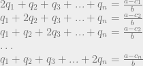
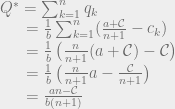
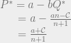
The first observation is that the behavior of the market under monopoly looks very different from the case of perfect competition. For one thing, notice that the price under perfect competition is always going to be lower than the price under monopoly. This is a nice demonstration of the so-called monopoly markup. The quantity $a$ intuitively corresponds to the highest possible price you could get for the product (the most that the highest bidder would pay). And the quantity $c$ , the production cost, is the lowest possible price at which the product would be sold. So the monopoly price is the average of the highest price you could get for the good and the lowest price at which it could be sold.

The flip side of the monopoly markup is that less of the good is produced and sold under a monopoly than under perfect competition. There are trades that could be happening (trades which would be mutually beneficial!) which do not occur. Think about it: the monopoly price is halfway between the cost of production and the highest bidder’s price. This means that there are a bunch of people that would buy the product at above the cost of production but below the monopoly price. And since the price they would buy it for is above the cost of production, this would be a profitable exchange for both sides! But alas, the monopoly doesn’t allow these trades to occur, as it would involve lowering the price for everybody, including those who are willing to pay a higher price, and thus decreasing net profit.

Things change as soon as another firm joins the market. This firm can profitably sell the good at a lower price than the monopoly price and snatch up all of their business. This introduces a downward pressure on the price. Here’s the exact solution for the case of duopoly.

Duopoly: n = 2
$q_1 = \frac{1}{3b} (a - 2c_1 + c_2) \\ q_2 = \frac{1}{3b} (a + c_1 - 2c_2) \\ Q^* = \frac{1}{3b} (2a - c_1 - c_2) \\ P^* = \frac{1}{3} (a + c_1 + c_2) \\ \Pi_1^* = \frac{1}{3b} (a - 2c_1 + c_2)^2 \\ \Pi_2^* = \frac{1}{3b} (a + c_1 - 2c_2)^2 \\$

Interestingly, in the duopoly case the market price still rests at a value above the marginal cost of production for either firm. As more and more firms enter the market, competition pushes the price down further and further until, in the limit of perfect competition, it converges to the cost of production.

The implication of this is that in the limit of perfect competition, firms do not make any profit! This may sound a little unintuitive, but it’s the inevitable consequence of the line of argument above. If a bunch of companies were all making some profit, then their price is somewhere above the cost of production. But this means that one company could slightly lower its price, thus snatching up all the customers and making massively more money than its competitors. So its competitors will all follow suit, pushing down their prices to get back their customers. And in the end, all the firms will have just decreased their prices and their profits, even though every step in the sequence appeared to be the rational and profitable action by each firm! This is just an example of a coordination problem. If the companies could all just agree to hold their price fixed at, say, the monopoly price, then they’d all be better off. But each individual has a strong monetary incentive to lower their price and gather all the customers. So the price will drop and drop until it can drop no more (that is, until it has reached the cost of production, at which point it is no longer profitable for a company to lower their price).

This implies that in some sense, the limit of perfect competition is the best possible outcome for consumers and the worst outcome for producers. Every consumer that values the product above the cost of its production will get it, and they will all get it at the lowest possible price. So the consumer surplus will be enormous. And companies producing the product make no net profit; any attempt to do so immediately loses them their entire customer base. (In which case, what is the motivation for the companies to produce the product in the first place? This is known as the Bertrand paradox.)

We can also get the easier-to-solve special case where all firms have the same cost of production.

Equal Production Costs
$\forall k (c_k = c)$
$q_k^* = \frac{1}{n+1} \frac{a - c}{b} \\ Q^* = \frac{n}{n+1} \frac{a - c}{b} \\ P^* = \frac{a + nc}{n + 1} \\ \Pi^* = \frac{1}{b} \left( \frac{a - c}{n+1} \right)^2$

It’s curious that in the Cournot model, prices don’t immediately drop to production levels as soon you go from a monopoly to a duopoly. After all, the intuitive argument I presented before works for two firms: if both firms are pricing the goods at any value above zero, then each stands to gain by lowering the price a slight bit and getting all the customers. And this continues until the price settles at the cost of production. We didn’t build in any ability of the firms to collude to the model, so what gives? What the Cournot model tells us is certainly more realistic (we don’t expect a duopoly to behave like a perfectly competitive market), but where does this realism come from?

The answer is that in a certain sense we did build in collusion between firms from the start, in the form of agreement on what price to sell at. Notice that our model did not allow different firms to set different prices. In this model, firms compete only on quantity of goods sold, not prices. The price is set automatically by the consumer demand function, and no single individual can unilaterally change their price. This constraint is what gives us the more realistic-in-character results that we see, and also what invalidates the intuitive argument I’ve made here.

One final observation. Consider the following procedure. You line up a representative from each of the n firms, as well as the highest bidder for the product (representing the highest price at which the product could be sold). Each of the firms states their cost of production (the lowest they could profitably bring the price to), and the highest bidder states the amount that he values the product (the highest price at which he would still buy it). Now all of the stated costs are averaged, and the result is set as the market price of the good. Turns out that this procedure gives exactly the market price that the linear Cournot model predicts! This might be meaningful or just a curious coincidence. But it’s quite surprising to me that the slope of the demand curve ( $b$ ) doesn’t show up at all in the ultimate market price, only the value that the highest bidder puts on the product!

Building an analog calculator

November 25, 2019 ~ squarishbracket ~ 1 Comment

Op-amps are magical little devices that allow us to employ the laws of electromagnetism for our purposes, giving us the power to do ultimately any computation using physics. To explain this, we need to take three steps: first transistors, then differential amplifiers, and then operational amplifiers. The focus of this post will be on purely analog calculations, as that turns out to be the most natural type of computation you get out of op amps.

1. Transistor

Here’s a transistor:

It has three ports, named (as labelled) the base, the collector and the emitter. Intuitively, you can think about the base as being like a dial that sensitively controls the flow of large quantities of current from the collector to the emitter. This is done with only very small trickles of current flowing into the base.

More precisely, a transistor obeys the following rules:

The transistor is ON if the voltage at the collector is higher than the voltage at the emitter. It is OFF otherwise.
When the transistor is in the ON state, which is all we’ll be interested in, the following regularities are observed:
1. Current flows along only two paths: base-to-emitter and collector-to-emitter. A transistor does not allow current to flow from the emitter to either the collector or the base.
2. The current into the collector is proportional to the current into the base, with a constant of proportionality labelled β whose value is determined by the make of the transistor. β is typically quite large, so that the current into the collector is much larger than the current into the base.
3. The voltage at the emitter is 0.6V less than the voltage at the base.

Combined, these rules allow us to solve basic transistor circuits. Here’s a basic circuit that amplifies input voltages using a transistor:

Applying the above rules, we derive the following relationship between the input and output voltages:

The +15V port at the top is important for the functioning of the amplifier because of the first rule of transistors, regarding when they are ON and OFF. If we just had it grounded, then the voltage at the collector would be negative (after the voltage drop from the resistor), so the transistor would switch off. Having the voltage start at +15V allows V_C to be positive even after the voltage drop at the resistor (although it does set an upper bound on the input currents for which the circuit will still operate).

And the end result is that any change in the input voltage will result in a corresponding change in the output voltage, amplified by a factor of approximately -R_C/R_E. Why do we call this amplification? Well, because we can choose whatever values of resistance for R_C and R_E that we want! So we can make R_C a thousand times larger than R_E, and we have created an amplifier that takes millivolt signals to volt signals. (The amplification tops out at +15V, because a signal larger than that would result in the collector voltage going negative and the transistor turning off.)

Ok, great, now you’re a master of transistor circuits! We move on to Step 2: the differential amplifier.

2. Differential Amplifier

A differential amplifier is a circuit that amplifies the difference between two voltages and suppresses the commonalities. Here’s how to construct a differential amplifier from two transistors:

Let’s solve this circuit explicitly:

V_in= 0.6 + R_Ei_E+ R_f (i_E+ i_E’)
V_in’ = 0.6 + R_Ei_E’ + R_f(i_E+ i_E’)

∆(V_in – V_in’) = R_E(i_E– i_E’) = R_E(β+1)(i_B – i_B’)
∆(V_in + V_in’) = (R_E + 2R_f)(i_E + i_E’) = (R_E + 2R_f)(β+1)(i_B + i_B’)

V_out = 15 – R_Ci_CV_out’ = 15 – R_C i_C’

∆(V_out – V_out’) = – R_C(i_C– i_C’) = – R_Cβ (i_B– i_B’)
∆(V_out + V_out’) = – R_C(i_C+ i_C’) = – R_C β (i_B+ i_B’)

A_DM = Differential Amplification = ∆(V_out – V_out’) / ∆(V_in– V_in’) = -β/(β+1) R_C/R_E
A_CM = “Common Mode” Amplification = ∆(V_out + V_out’) / ∆(V_in+ V_in’) = -β/(β+1) R_C/(R_E+ 2R_f)

We can solve this directly for changes in one particular output voltage:

∆V_out = A_DM ∆(V_in– V_in‘) + A_CM ∆(V_in+ V_in‘)

To make a differential amplifier, we require that A_DM be large and A_CM be small. We can achieve this if R_f >> R_C>> R_C. Notice that since the amplification is a function of the ratio of our resistors, we can easily make the amplification absolutely enormous.

Here’s one way this might be useful: say that Alice wants to send a signal to Bob over some distance, but there is a source of macroscopic noise along the wire connecting the two. Perhaps the wire happens to pass through a region in which large magnetic disturbances sometimes occur. If the signal is encoded in a time-varying voltage on Alice’s end, then what Bob gets may end up being a very warped version of what Alice sent.

But suppose that instead Alice sends Bob two signals, one with the original message and the other just a static fixed voltage. Now the difference between the two signals represents Alice’s message. And crucially, if these two signals are sent on wires that are right side-by-side, then they will pick up the same noise!

75223836_434765827156596_5577175764417118208_n

This means that while the original message will be warped, so will the static signal, and by roughly the same amount! Which means that the difference between the two signals will still carry the information of the original message. This allows Alice to communicate with Bob through the noise, so long as Bob takes the two wires on his end and plugs them into a differential amplifier to suppress the common noise factor.

3. Operational Amplifier

To make an operational amplifier, we just need to make some very slight modifications to our differential amplifier. The first is that we’ll make our amplification as large as possible. We can get this by putting multiple stages of differential amplifiers side by side (so if your differential amplifier amplifies by 100, two of them will amplify by 10,000, and three by 1,000,000).

What’ll happen now if we send in two voltages, with V_in very slightly larger than V_in‘? Well, suppose that the difference is on the order of a single millivolt (mV). Then the output voltage will be on the order of 1 mV multiplied by our amplication factor of 1,000,000. This will be around 1000V. So… do we expect to get out an output signal of 1000V? No, clearly not, because our maximum possible voltage at the output is +15V! We can’t create energy from nowhere. Remember that the output voltage V_out is equal to 15V – R_Ci_C, and that the transistor only accepts current traveling from the collector to the emitter, not the other way around. This means that i_C cannot be negative, so V_out cannot be larger that +15V. In addition, we know that V_out cannot be smaller than 0V (as this would turn off the transistor via Rule 1 above).

What this all means is that if V_in is even the slightest bit smaller than V_in‘, V_out will “max out”, jumping to the peak voltage of +15V (remember that A_DM is negative). And similarly, if V_in is even the slightest bit larger than V_in‘, then V_out will bottom out, dropping to 0V. The incredible sensitivity of the instrument is given to us by the massive amplification factor, so that it will act as a binary measurement of which of the voltages is larger, even if that difference is just barely detectable. Often, the bottom voltage will be set to -15V rather than ground (0V), so that the signal we get out is either +15V (if V_in is smaller than V_in‘) or -15V (if V_in is greater than V_in‘). That way, perfect equality of the inputs will be represented as 0V. That’s the convention we’ll use for the rest of the post. Also, instead of drawing out the whole diagram for this modified differential amplifier, we will use the following simpler image:

Ok, we’re almost to an operational amplifier. The final step is to apply negative feedback!

78675994_2469781120006676_3367768905735995392_n

What we’re doing here is just connecting the output voltage to the V_in‘ input. Let’s think about what this does. Suppose that V_in is larger than V_in‘. Then V_out will quickly become negative, approaching -15V. But as V_out decreases, so does V_in‘! So V_in‘ will decrease, getting closer to V_in. Once it passes V_in, the quantity V_in– V_in‘ suddenly becomes negative, so V_out will change direction, becoming more positive and approaching +15V. So V_in‘ will begin to increase! This will continue until it passes V_in again, at which point V_out will change signs again and V_in‘ will start decreasing. The result of this process will be that no matter what V_in‘ starts out as, it will quickly adjust to match V_in to a degree dictated by the resolution of our amplifier. And we’ve already established that the amplifier can be made to have an extremely high resolution. So this device serves as an extremely precise voltage-matcher!

This device, a super-sensitive differential amplifier with negative feedback, is an example of an operational amplifier. It might not be immediately obvious to you what’s so interesting or powerful about this device. Sure it’s very precise, but all it does is match voltages. How can we leverage this to get actually interesting computational behavior? Well, that’s the most fun part!

4. Let’s Compute!

Let’s start out by seeing how an op-amp can be used to do calculus. Though this might seem like an unusually complicated starting place, doing calculus with op amps is significantly easier and simpler than doing something like multiplication.

As we saw in the last section, if we simply place a wire between V_out and V_in‘ (the input labelled with a negative sign on the diagram), then we get a voltage matcher. We get more interesting behavior if we place other circuit components along this wire. The negative feedback still exists, which means that the circuit will ultimately stabilize to a state in which the two inputs are identical, and where no current is flowing into the op-amp. But now the output voltage will not just be zero.

Let’s take a look at the following op-amp circuit:

Notice that we still have negative feedback, because the V_– input is connected to the output, albeit not directly. This means that the two inputs to the op amp must be equal, and since V₊ is grounded, the other must be at 0V as well. It also means that no current is flowing into the op amp, as current only flows in while the system is stabilizing.

Those two pieces of information – that the input voltages are equal and that no current flows through the device – are enough to allow us to solve the circuit.

78702668_568111487351368_4817792612675092480_n-3402953477-1574653952986.jpg

And there we have it, a circuit that takes in a voltage function that changes with time and outputs the integral of this function! A natural question might be “integral from what to what”? The answer is just: the integral from the moment the circuit is connected to the present! As soon as the circuit is connected it begins integrating.

Alright, now let’s just switch the capacitor and resistor in the circuit:

See if you can figure out for yourself what this circuit does!

…

Alright, here’s the solution.

We have a differentiator! Feed in some input voltage, and you will get out a precise measurement of the rate of change of this voltage!

I find it pretty amazing that doing integration and differentiation is so simple and natural. Addition is another easy one:

We can use diodes to produce exponential and logarithm calculators. We utilize the ideal diode equation:

76710826_595060124565198_3738884638802706432_n

The logarithm can now be used to produce circuits for calculating exponentials and logarithms:

78272557_661889637548819_7805558089259679744_n

Again, these are all fairly simple-looking circuits. But now let’s look at the simplest way of computing multiplication using an op amp. Schematically, it looks like this:

And here’s the circuit in full detail:

76759967_2648350875451816_1144785316129800192_n

There’s another method besides this one that you can use to do multiplication, but it’s similarly complicated. It’s quite intriguing that multiplication turns out to be such an unnatural thing to get nature to do to voltages, while addition, exponentiation, integration, and the rest are so simple.

What about boolean logic? Well, it turns out that we already have a lot of it. Our addition corresponds to an OR gate if the input voltages are binary signals. We also already have an AND gate, because we have multiplication! And depending on our choice of logic levels (which voltage corresponds to True and which corresponds to False), we can really easily sketch a circuit that does negation:

And of course if we have NOT and we have AND, then we have NAND, and if we have NAND, then we have all the rest of binary logic. We can begin to build flip-flop gates out of the NAND gates to get simple memory cells, and we’re on our way to Turing-completeness!

Complex numbers in physics

November 23, 2019November 23, 2019 ~ squarishbracket ~ Leave a comment

“You cannot observe an imaginary number in reality.” Have you ever heard this claim before? It has a nice ring to it, and sounds almost tautological. I’ve personally heard the claim made by several professors of physics, alongside a host of less qualified people. So let’s take a close look at it and see if it holds up to scrutiny. Can you in fact observe imaginary numbers in reality?

First of all, let’s ask a much simpler sounding question. Can you ever observe a real number in reality? Well, yeah. Position, time, charge, mass, and so on; pretty much any physical quantity you name can be represented by real numbers. But if we’re going to be pedantic, when we measure the position of a particle, we are not technically observing a number. We are observing a position, a physical quantity, which we find has a useful representation as a real number. Color is another physical phenomena that is usually represented mathematically as a real number (the frequency of emitted light). But we do not necessarily want to say that color is a number. No, we say that color is a physical phenomena, which we find is usefully described as a real number.

More specifically, we have some physical phenomena whose structure contains many similarities to the abstract structure of these mathematical objects known as real numbers, so it behooves us to translate statements about the phenomena over to the platonic realm of math, where the work we do is precise and logically certain. Once we have done the mathematical manipulations we desire to get useful results, we translate our statements about numbers back into statements about the physical phenomena. There are really just two possible failure points in this process. First, it might be that the mathematical framework actually doesn’t have the same structure as the physical phenomena we have chosen it to describe. And second, it might be that the mathematical manipulations we do once we have translated our physical statements into mathematical statements contain some error (like maybe we accidentally divided by zero or something).

So on one (overly literal) interpretation, when somebody asks whether a certain abstract mathematical object exists in reality, the answer is always no. Numbers and functions and groups and rings don’t exist in reality, because they are by definition abstract objects, not concrete ones. But this way of thinking about the relationship between math and physics does give us a more useful way to answer the question. Do real numbers exist in reality? Well, yes, they exist insofar as their structure is mirrored in the structure of some real world phenomena! If we’re being careful with our language, we might want to say that real numbers are instantiated in reality instead of saying that they exist.

So, are imaginary numbers instantiated in reality? Well, yes, of course they are! The wave function in quantum mechanics is an explicitly complex entity — try doing quantum mechanics with only real-valued wave functions, and you will fail, dramatically. The existence of imaginary values of the wave function is absolutely necessary in order to get an adequate description of our reality. So if you believe quantum mechanics, then you believe that imaginary numbers are actually embedded in the structure of the most fundamental object there is: the wave function of the universe.

A simpler example: any wave-like phenomena is best described in the language of complex numbers. A ripple in the water is described as a complex function of position and time, where the complex phase of the function represents the propagation of the wave through space and time. Any time you see a wave-like phenomena (by which I mean any process that is periodic, including something as prosaic as a ticking clock), you are looking at a physical process that really nicely mirrors the structure of complex numbers.

Now we’ll finally get to the main point of this post, which is to show off a particularly elegant and powerful instance of complex numbers applying to physics. This example is in the realm of electromagnetism, specifically the approximation of electromagnetism that we use when we talk about circuits, resistors, capacitors, and so on.

Suppose somebody comes up to you in the street, hands you the following circuit diagram, and asks you to solve it:

If you’ve never studied circuits before, you might stare at it blankly for a moment, then throw your hands up in puzzlement and give them back their sheet of paper.

If you’ve learned a little bit about circuits, you might stare at it blankly for a few moments, then write down some complicated differential equations, stare at them for a bit, and then throw your hands up in frustration and hand the sheet back to them.

And if you know a lot about circuits, then you’ll probably smile, write down a few short lines of equations involving imaginary numbers, and hand back the paper with the circuit solved.

Basically, the way that students are initially taught to solve circuits is to translate them into differential equations. These differential equations quickly become immensely difficult to solve (as differential equations tend to do). And so, while a few simple circuits are nicely solvable with this method, any interesting circuits that do nontrivial computations are at best a massive headache to solve with this method, and at worst actually infeasible.

This is the real numbers approach to circuits. But it’s not the end of the story. There’s another way! A better and more beautiful way! And it uses complex numbers.

Here’s the idea: circuits are really easy to solve if all of your circuit components are just resistors. For a resistor, the voltage across it is just linearly proportional to the current through it. No derivatives or integrals required, we just use basic algebra to solve one from the other. Furthermore, we have some nice little rules for simplifying complicated-looking resistor circuits by finding equivalent resistances.

The problem is that interesting circuits don’t just involve resistors. They also contain things like inductors and capacitors. And these circuit elements don’t have that nice linear relationship between current and voltage. For capacitors, the relationship is between voltage and the integral of current. And for inductors, the relationship is between voltage and the derivative of current. Thus, a circuit involving a capacitor, a resistor, and an inductor, is going to be solved by an equation that involves the derivative of current, the current itself, and the integral of current. In other words, a circuit involving all three types of circuit elements is in general going to be solved by a second-order differential equation. And those are a mess.

The amazing thing is that if instead of treating current and voltage as real-valued functions, you treat them as complex-valued functions, what you find is that capacitors and inductors behave exactly like resistors. Voltage and current become related by a simple linear equation once more, with no derivatives or integrals involved. And the distinguishing characteristic of a capacitor or an inductor is that the constant of proportionality between voltage and current is an imaginary number instead of a real number. More specifically, a capacitor is a circuit element for which voltage is equal to a negative imaginary number times the current. An inductor is a circuit element for which voltage is equal to a positive imaginary number times the current. And a resistor is a circuit element for which voltage is equal to a positive real number times the current.

Suppose our voltage is described by a simple complex function: V₀exp(iωt). Then we can describe the relationship between voltage and current for each of these circuit elements as follows:

Notice that now the equations for all three circuit components look just like resistors! Just with different constants of proportionality relating voltage to current. We can even redraw our original diagrams to make the point:

Fourier showed that any function whatsoever can be described as a sum of functions that look like Vo exp(iωt). And there’s a nice theorem called the superposition theorem that allows us to use this to solve any circuit, no matter what the voltage is.

So, let’s go back to our starting circuit.

What we can now do is just redraw it, with all capacitors and inductors substituted for resistors with imaginary resistances:

This may look just as complicated as before, but it’s actually much much simpler. We can use the rules for reducing resistor equations to solve an immensely simpler circuit:

Our circuit is now much simpler, but the original complexity had to be offloaded somewhere. As you can see, it’s been offloaded onto the complex (in both senses of the word) value of the resistance of our simplified circuit. But this type of complexity is much easier to deal with, because it’s just algebra, not calculus! To solve the current in our circuit now, we don’t need to solve a single differential equation, we just have to do some algebraic rearranging of terms. We’ll give the final equivalent resistance the name “Z”.

Now suppose that our original voltage was just the real part of V (that is, V₀cos(ωt)). Then the current will also be the real part of I. And if our original voltage was just the imaginary part of V, then the current will be the imaginary part of I. And there we have it! We’ve solved our circuit without struggling over a single differential equation, simply by assuming that our quantities were complex numbers instead of real numbers.

This is one of my favorite examples of complex numbers playing an enormously important role in physics. It’s true that it’s a less clear-cut example of complex numbers being necessary to describe a physical phenomena, because we could have in principle done everything with purely real-valued functions by solving some differential equations, but it also highlights the way in which accepting a complex view of the world can simplify your life.

The Central Paradox of Statistical Mechanics: The Problem of The Past

September 28, 2019September 30, 2019 ~ squarishbracket ~ 2 Comments

This is the third part in a three-part series on the foundations of statistical mechanics.

The Necessity of Statistical Mechanics for Getting Macro From Micro
Is The Fundamental Postulate of Statistical Mechanics A Priori?
The Central Paradox of Statistical Mechanics: The Problem of The Past

— — —

What I’ve argued for so far is the following set of claims:

To successfully predict the behavior of macroscopic systems, we need something above and beyond the microphysical laws.
This extra thing we need is the fundamental postulate of statistical mechanics, which assigns a uniform distribution over the region of phase space consistent with what you know about the system. This postulate allows us to prove all the things we want to say about the future, such as “gases expand”, “ice cubes melt”, “people age” and so on.
This fundamental postulate is not justifiable on a priori grounds, as it is fundamentally an empirical claim about how frequently different micro states pop up in our universe. Different initial conditions give rise to different such frequencies, so that a claim to a priori access to the fundamental postulate is a claim to a priori access to the precise details of the initial condition of the universe.

There’s just one problem with all this… apply our postulate to the past, and everything breaks.

Notice that I said that the fundamental postulate allows us to prove all the things we want to say about the future. That wording was chosen carefully. What happens if you try to apply the microphysical laws + the fundamental postulate to predict the past of some macroscopic system? It turns out that all hell breaks loose. Gases spontaneously contract, ice cubes form from puddles of water, and brains pop out of thermal equilibrium.

Why does this happen? Very simply, we start with two fully time reversible premises (the microphysical laws and the fundamental postulate). We apply it to present knowledge of some state, the description of which does not specify a special time direction. So any conclusion we get must as a matter of logic be time reversible as well! You can’t start with premises that treat the past as the mirror image of the future, and using just the rules of logical equivalence derive a conclusion that treats the past as fundamentally different from the future. And what this means is that if you conclude that entropy increases towards the future, then you must also conclude that entropy increases towards the past. Which is to say that we came from a higher entropy state, and ultimately (over a long enough time scale and insofar as you think that our universe is headed to thermal equilibrium) from thermal equilibrium.

Let’s flesh this argument out a little more. Consider a half-melted ice cube sitting in the sun. The microphysical laws + the fundamental postulate tell us that the region of phase space consisting of states in which the ice cube is entirely melted is much much much larger than the region of phase space in which it is fully unmelted. So much larger, in fact, that it’s hard to express using ordinary English words. This is why we conclude that any trajectory through phase space that passes through the present state of the system (the half-melted cube) is almost certainly going to quickly move towards the regions of phase space in which the cube is fully melted. But for the exact same reason, if we look at the set of trajectories that pass through the present state of the system, the vast vast vast majority of them will have come from the fully-melted regions of phase space. And what this means is that the inevitable result of our calculation of the ice cube’s history will be that a few moments ago it was a puddle of water, and then it spontaneously solidified and formed into a half-melted ice cube.

This argument generalizes! What’s the most likely past history of you, according to statistical mechanics? It’s not that the solar system coalesced from a haze of gases strewn through space by a past supernova, such that a planet would form in the Goldilocks zone and develop life, which would then gradually evolve through natural selection to the point where you are sitting in whatever room you’re sitting in reading this post. This trajectory through phase space is enormously unlikely. The much much much more likely past trajectory of you through phase space is that a little while ago you were a bunch of particles dispersed through a universe at thermal equilibrium, which happened to spontaneously coalesce into a brain that has time to register a few moments of experience before dissipating back into chaos. “What about all of my memories of the past?” you say. As it happens the most likely explanation of these memories is not that they are veridical copies of real happenings in the universe but illusions, manufactured from randomness.

Basically, if you buy everything I’ve argued in the first two parts, then you are forced to conclude that the universe is most likely near thermal equilibrium, with your current experience of it arising as a spontaneous dip in entropy, just enough to produce a conscious brain but no more. There are at least two big problems with this view.

Problem 1: This conclusion is, we think, extremely empirically wrong! The ice cube in front of you didn’t spontaneously form from a puddle of water, uncracked eggs weren’t a moment ago scrambled, and your memories are to some degree veridical. If you really believe that you are merely a spontaneous dip in entropy, then your prediction for the next minute will be the gradual dissolution of your brain and loss of consciousness. Now, wait a minute and see if this happens. Still here? Good!

Problem 2: The conclusion cannot be simultaneously believed and justified. If you think that you’re a thermal fluctuation, then you shouldn’t credit any of your memories as telling you anything about the world. But then your whole justification to coming to the conclusion in the first place (the experiments that led us to conclude that physics is time-reversible and that the fundamental postulate is true) is undermined! Either you believe it without justification, or you don’t believe despite justification. Said another way, no reflective equilibrium exists at an entropy minimum. David Albert calls this peculiar epistemic state cognitively unstable, as it’s not clear where exactly it should leave you.

Reflect for a moment on how strange of a situation we are in here. Starting from very basic observations of the world, involving its time-reversibility on the micro scale and the increase in entropy of systems, we see that we are inevitably led to the conclusion that we are almost certainly thermal fluctuations, brains popping out of the void. I promise you that no trick has been pulled here, this really is the state of the philosophy of statistical mechanics! The big issue is how to deal with this strange situation.

One approach is to say the following: Our problem is that our predictions work towards the future but not the past. So suppose that we simply add as a new fundamental postulate the proposition that long long ago the universe had an incredibly low entropy. That is, suppose that instead of just starting with the microphysical laws and the fundamental postulate of statistical mechanics, we added a third claims: the Past Hypothesis.

The Past Hypothesis should be understood as an augmentation of our Fundamental Postulate. Taken together, the two postulates say that our probability distribution over possible microstates should not be uniform over phase space. Instead, it should be what you get when you take the uniform distribution, and then condition on the distant past being extremely low entropy. This process of conditioning clearly preferences one direction of time over the other, and so the symmetry is broken.

It’s worth reflecting for a moment on the strangeness of the epistemic status of the Past Hypothesis. It happens that we have over time accumulated a ton of observational evidence for the occurrence of the Big Bang. But none of this evidence has anything to do with our reasons for accepting the Past Hypothesis. If we buy the whole line of argument so far, our conclusion that something like a Big Bang occurred becomes something that we are forced to believe for deep logical reasons, on pain of cognitive instability and self-undermining belief. Anybody that denies that the Big Bang (or some similar enormously low-entropy past state) occurred has to contend with their view collapsing in self-contradiction upon observing the physical laws!

Is The Fundamental Postulate of Statistical Mechanics A Priori?

September 24, 2019September 30, 2019 ~ squarishbracket ~ 6 Comments

This is the second part in a three-part series on the foundations of statistical mechanics.

The Necessity of Statistical Mechanics for Getting Macro From Micro
Is The Fundamental Postulate of Statistical Mechanics A Priori?
The Central Paradox of Statistical Mechanics: The Problem of The Past

— — —

The fantastic empirical success of the fundamental postulate gives us a great amount of assurance that the postulate is good one. But it’s worth asking whether that’s the only reason that we should like this postulate, or if it has some solid a priori justification. The basic principle of “when you’re unsure, just distribute credences evenly over phase space” certainly strikes many people as highly intuitive and justifiable on a priori grounds. But there are some huge problems with this way of thinking, one of which I’ve already hinted at. Here’s a thought experiment that illustrates the problem.

There is a factory in your town that produces cubic boxes. All you know about this factory is that the boxes that they produce all have a volume between 0 m³ and 1 m³. You are going to be delivered a box produced by this factory, and are asked to represent your state of knowledge about the box with a probability distribution. What distribution should you use?

Suppose you say “I should be indifferent over all the possible boxes. So I should have a uniform distribution over the volumes from 0 m³ to 1 m³.” This might seem reasonable at first blush. But what if somebody else said “Yes, you should be indifferent over all the possible boxes, but actually the uniform distribution should be over the side lengths from 0 m to 1 m, not volumes.” This would be a very different probability distribution! For example, if the probability that the side length is greater than .5 m is 50%, then the probability that the volume is greater than (.5)³ = 1/8 is also 50%! Uniform over side length is not the same as uniform over volume (or surface area, for that matter). Now, how do you choose between a uniform distribution over volumes and a uniform distribution over side lengths? After all, you know nothing about the process that the factory is using to produce the boxes, and whether it is based off of volume or side length (or something else); all you know is that all boxes are between 0 m³ and 1 m³.

The lesson of this thought experiment is that the statement we started with (“I should be indifferent over all possible boxes”) was actually not even well-defined. There’s not just one unique measure over a continuous space, and in general the notion that “all possibilities are equally likely” is highly language-dependent.

The exact same applies to phase space, as position and momentum are continuous quantities. Imagine that somebody instead of talking about phase space, only talked about “craze space”, in which all positions become positions cubed, and all momentum values become natural logs of momentum. This space would still contain all possible microstates of your system. What’s more, the fundamental laws of nature could be rewritten in a way that uses only craze space quantities, not phase space quantities. And needless to say, being indifferent over phase space would not be the same as being indifferent over craze space.

Spend enough time looking at attempts to justify a unique interpretation of the statement “All states are equally likely”, when your space of states is a continuous infinity, and you’ll realize that all such attempts are deeply dependent upon arbitrary choices of language. The maximum information entropy probability distribution is afflicted with the exact same problem, because the entropy of your distribution is going to depend on the language you’re using to describe it! The entropy of a distribution in phase space is NOT the same as the entropy of the equivalent distribution transformed to craze space.

Let’s summarize this section. If somebody tells you that the fundamental postulate says that all microstates compatible with what you know about the macroscopic features of your system are equally likely, the proper response is something like “Equally likely? That sounds like you’re talking about a uniform distribution. But uniform over what? Oh, position and momentum? Well, why’d you make that choice?” And if they point out that the laws of physics are expressed in terms of position and momentum, you just disagree and say “No, actually I prefer writing the laws of physics in terms of position cubed and log momentum!” (Substitute in any choice of monotonic functions).

If they object on the grounds of simplicity, point out that position and momentum are only simple as measured from a standpoint that takes them to be the fundamental concepts, and that from your perspective, getting position and momentum requires applying complicated inverse transformations to your monotonic transformation of the chosen coordinates.

And if they object on the grounds of naturalness, the right response is probably something like “Tell me more about this ’naturalness’. How do you know what’s natural or unnatural? It seems to me that your choice of what physical concepts count as natural is a manifestation of deep selection pressures that push any beings whose survival depends on modeling and manipulating their surroundings towards forming an empirically accurate model of the macroscopic world. So that when you say that position is more natural than log(position), what I hear is that the fundamental postulate is a very useful tool. And you can’t use the naturalness of the choice of position to justify the fundamental postulate, when your perception of the naturalness of position is the result of the empirical success of the fundamental postulate!”

In my judgement, none of the a priori arguments work, and fundamentally the reason is that the fundamental postulate is an empirical claim. There’s no a priori principle of rationality that tells us that boxes of gases tend to equilibrate, because you can construct a universe whose initial microstate is such that its entire history is one of entropy radically decreasing, gases concentrating, eggs unscrambling, ice cubes unmelting, and so on. Why is this possible? Because it’s consistent with the microphysical laws that the universe started in an enormously low entropy configuration, so it’s gotta also be consistent with the microphysical laws for the entire universe to spend its entire lifetime decreasing in entropy. The general principle is: If you believe that something is physically possible, then you should believe its time-inverse is possible as well.

Let’s pause and take stock. What I’ve argued for so far is the following set of claims:

To successfully predict the behavior of macroscopic systems, we need something above and beyond the microphysical laws.
This extra thing we need is the fundamental postulate of statistical mechanics, which assigns a uniform distribution over the region of phase space consistent with what you know about the system. This postulate allows us to prove all the things we want to say about the future, such as “gases expand”, “ice cubes melt”, “people age” and so on.
This fundamental postulate is not justifiable on a priori grounds, as it is fundamentally an empirical claim about how frequently different microstates pop up in our universe. Different initial conditions give rise to different such frequencies, so that a claim to a priori access to the fundamental postulate is a claim to a priori access to the precise details of the initial condition of the universe.

There’s just one problem with all this… apply our postulate to the past, and everything breaks.

Up next: Why does statistical mechanics give crazy answers about the past? Where did we go wrong?

A Cognitive Instability Puzzle, Part 2

September 18, 2019September 18, 2019 ~ squarishbracket ~ 4 Comments

This is a follow of this previous post, in which I present three unusual cases of belief updating. Read it before you read this.

I find these cases very puzzling, and I don’t have a definite conclusion for any of them. They share some deep similarities. Let’s break all of them down into their basic logical structure:

Joe
Joe initially believes in classical logic and is certain of some other stuff, call it X.
An argument A exists that concludes that X can’t be true if classical logic is true.
If Joe believes classical logic, then he believes A.
If Joe believes intuitionist logic, then he doesn’t believe A.

Karl
Karl initially believes in God and is certain of some other stuff about evil, call it E.
An argument A exists that concludes that God can’t exist if E is true.
If Karl believes in God, then he believes A.
If Karl doesn’t believe in God, then he doesn’t believe A.

Tommy
Tommy initially believes in her brain’s reliability and is certain of some other stuff about her experiences, call it Q.
An argument A exists that concludes that hat her brain can’t be reliable if Q is true.
If Tommy believes in her brain’s reliability, then she believes A.
If Tommy doesn’t believe in her brain’s reliability, then she doesn’t believe A.

First of all, note that all three of these cases are ones in which Bayesian reasoning won’t work. Joe is uncertain about the law of the excluded middle, without which you don’t have probability theory. Karl is uncertain about the meaning of the term ‘evil’, such that the same proposition switches from being truth-apt to being meaningless when he updates his beliefs. Probability theory doesn’t accommodate such variability in its language. And Tommy is entertaining a hypothesis according to which she no longer accepts any deductive or inductive logic, which is inconsistent with Bayesianism in an even more extreme way than Joe.

The more important general theme is that in all three cases, the following two things are true: 1) If an agent believes A, then they also believe an argument that concludes -A. 2) If that agent believes -A, then they don’t believe the argument that concludes -A.

Notice that if an agent initially doesn’t believe A, then they have no problem. They believe -A, and also happen to not believe that specific argument concluding -A, and that’s fine! There’s no instability or self-contradiction there whatsoever. So that’s really not where the issue lies.

The mystery is the following: If the only reason that an agent changed their mind from A to -A is the argument that they no longer buy, then what should they do? Once they’ve adopted the stance that A is false, should they stay there, reasoning that if they accept A they will be led to a contradiction? Or should they jump back to A, reasoning that the initial argument that led them there was flawed?

Said another way, should they evaluate the argument against A from their own standards, or from A’s standards? If they use their own standards, then they are in an unstable position, where they jump back and forth between A and -A. And if they always use A’s standards… well, then we get the conclusion that Tommy should believe herself to be a Boltzmann brain. In addition, if they are asked why they don’t believe A, then they find themselves in the weird position of giving an explanation in terms of an argument that they believe to be false!

I find myself believing that either Joe should be an intuitionist, Karl an atheist, and Tommy a radical skeptic, OR Joe a classical-logician, Karl a theist, and Tommy a reliability-of-brain-believer-in. That is, it seems like there aren’t any significant enough disanalogies between these three cases to warrant concluding one thing in one case and then going the other direction in another.

Logic, Theism, and Boltzmann Brains: On Cognitively Unstable Beliefs

September 16, 2019September 18, 2019 ~ squarishbracket ~ 7 Comments

First case

Propositional logic accepts that the proposition A∨-A is necessarily true. This is called the law of the excluded middle. Intuitionist logic differs in that it denies this axiom.

Suppose that Joe is a believer in propositional logic (but also reserves some credence for intuitionist logic). Joe also believes a set of other propositions, whose conjunction we’ll call X, and has total certainty in X.

One day Joe discovers that a contradiction can be derived from X, in a proof that uses the law of the excluded middle. Since Joe is certain that X is true, he knows that X isn’t the problem, and instead it must be the law of the excluded middle. So Joe rejects the law of the excluded middle and becomes an intuitionist.

The problem is, as an intuitionist, Joe now no longer accepts the validity of the argument that starts at X and concludes -X! Why? Because it uses the law of the excluded middle, which he doesn’t accept.

Should Joe believe in propositional logic or intuitionism?

Second case

Karl is a theist. He isn’t absolutely certain that theism is correct, but holds a majority of his credence in theism (and the rest in atheism). Karl is also 100% certain in the following claim: “If atheism is true, then the concept of ‘evil’ is meaningless”, and believes that logically valid arguments cannot be made using meaningless concepts.

One day somebody presents the problem of evil to Karl, and he sees it as a crushing objection to theism. He realizes that theism, plus some other beliefs about evil that he’s 100% confident in, leads to a contradiction. So since he can’t deny these other beliefs, he is led to atheism.

The problem is, as an atheist, Karl no longer accepts the validity of the argument that starts at theism and concludes atheism! Why? Because the arguments rely on using the concept of ‘evil’, and he is now certain that this concept is meaningless, and thus cannot be used in logically valid arguments.

Should Karl be a theist or an atheist?

Third case

Tommy is a scientist, and she believes that her brain is reliable. By this, I mean that she trusts her ability to reason both deductively and inductively. However, she isn’t totally certain about this, and holds out a little credence for radical skepticism. She is also totally certain about the content of her experiences, though not its interpretation (i.e. if she sees red, she is 100% confident that she is experiencing red, although she isn’t necessarily certain about what in the external world is causing the experience).

One day Tommy discovers that reasoning deductively and inductively from her experiences leads her to a model of the world that entails that her brain is actually a quantum fluctuation blipping into existence outside the event hole of a black hole. She realizes that this means that with overwhelmingly high probability, her brain is not reliable and is just producing random noise uncorrelated with reality.

The problem is, if Tommy believes that her brain is not reliable, then she can no longer accept the validity of the argument that led her to this position! Why? Well, she no longer trusts her ability to reason deductively or inductively. So she can’t accept any argument, let alone this particular one.

What should Tommy believe?

— — —

How are these three cases similar and different? If you think that Joe should be an intuitionist, or Karl an atheist, then should Tommy believe herself to be a black hole brain? Because it turns out that many cosmologists have found themselves to be in a situation analogous to Case 3! (Link.) I have my own thoughts on this, but I won’t share them for now.

How will quantum computing impact the world?

May 15, 2019May 15, 2019 ~ squarishbracket ~ Leave a comment

A friend of mine recently showed me an essay series on quantum computers. These essays are fantastically well written and original, and I highly encourage anybody with the slightest interest in the topic to check them out. They are also interesting to read from a pedagogical perspective, as experiments in a new style of teaching (self-described as an “experimental mnemonic medium”).

There’s one particular part of the post which articulated the potential impact of quantum computing better than I’ve seen it articulated before. Reading it has made me update some of my opinions about the way that quantum computers will change the world, and so I want to post that section here with full credit to the original authors Michael Nielsen and Andy Matuschak. Seriously, go to the original post and read the whole thing! You won’t regret it.

No, really, what are quantum computers good for?

It’s comforting that we can always simulate a classical circuit – it means quantum computers aren’t slower than classical computers – but doesn’t answer the question of the last section: what problems are quantum computers good for? Can we find shortcuts that make them systematically faster than classical computers? It turns out there’s no general way known to do that. But there are some interesting classes of computation where quantum computers outperform classical.

Over the long term, I believe the most important use of quantum computers will be simulating other quantum systems. That may sound esoteric – why would anyone apart from a quantum physicist care about simulating quantum systems? But everybody in the future will (or, at least, will care about the consequences). The world is made up of quantum systems. Pharmaceutical companies employ thousands of chemists who synthesize molecules and characterize their properties. This is currently a very slow and painstaking process. In an ideal world they’d get the same information thousands or millions of times faster, by doing highly accurate computer simulations. And they’d get much more useful information, answering questions chemists can’t possibly hope to answer today. Unfortunately, classical computers are terrible at simulating quantum systems.

The reason classical computers are bad at simulating quantum systems isn’t difficult to understand. Suppose we have a molecule containing atoms – for a small molecule, may be – $10$ , for a complex molecule it may be hundreds or thousands or even more. And suppose we think of each atom as a qubit (not true, but go with it): to describe the system we’d need $2^n$ different amplitudes, one amplitude for each $n$ –bit computational basis state, e.g., $\dots ⟩$ .

Of course, atoms aren’t qubits. They’re more complicated, and we need more amplitudes to describe them. Without getting into details, the rough scaling for an $n$ –atom molecule is that we need $k^n$ amplitudes, where $k \geq 2$ . The value of k depends upon context – which aspects of the atom’s behavior are important. For generic quantum simulations may be in the hundreds or more.

That’s a lot of amplitudes! Even for comparatively simple atoms and small values of $n$ , it means the number of amplitudes will be in the trillions. And it rises very rapidly, doubling or more for each extra atom. If $k = 100$ , then even $10$ atoms will require 100 million trillion amplitudes. That’s a lot of amplitudes for a pretty simple molecule.

The result is that simulating such systems is incredibly hard. Just storing the amplitudes requires mindboggling amounts of computer memory. Simulating how they change in time is even more challenging, involving immensely complicated updates to all the amplitudes.

Physicists and chemists have found some clever tricks for simplifying the situation. But even with those tricks simulating quantum systems on classical computers seems to be impractical, except for tiny molecules, or in special situations. The reason most educated people today don’t know simulating quantum systems is important is because classical computers are so bad at it that it’s never been practical to do. We’ve been living too early in history to understand how incredibly important quantum simulation really is.

That’s going to change over the coming century. Many of these problems will become vastly easier when we have scalable quantum computers, since quantum computers turn out to be fantastically well suited to simulating quantum systems. Instead of each extra simulated atom requiring a doubling (or more) in classical computer memory, a quantum computer will need just a small (and constant) number of extra qubits. One way of thinking of this is as a loose quantum corollary to Moore’s law:

The quantum corollary to Moore’s law: Assuming both quantum and classical computers double in capacity every few years, the size of the quantum system we can simulate scales linearly with time on the best available classical computers, and exponentially with time on the best available quantum computers.

In the long run, quantum computers will win, and win easily.

The punchline is that it’s reasonable to suspect that if we could simulate quantum systems easily, we could greatly speed up drug discovery, and the discovery of other new types of materials.

I will risk the ire of my (understandably) hype-averse colleagues and say bluntly what I believe the likely impact of quantum simulation will be: there’s at least a 50 percent chance quantum simulation will result in one or more multi-trillion dollar industries. And there’s at least a 30 percent chance it will completely change human civilization. The catch: I don’t mean in 5 years, or 10 years, or even 20 years. I’m talking more over 100 years. And I could be wrong.

What makes me suspect this may be so important?

For most of history we humans understood almost nothing about what matter is. That’s changed over the past century or so, as we’ve built an amazingly detailed understanding of matter. But while that understanding has grown, our ability to control matter has lagged. Essentially, we’ve relied on what nature accidentally provided for us. We’ve gotten somewhat better at doing things like synthesizing new chemical elements and new molecules, but our control is still very primitive.

We’re now in the early days of a transition where we go from having almost no control of matter to having almost complete control of matter. Matter will become programmable; it will be designable. This will be as big a transition in our understanding of matter as the move from mechanical computing devices to modern computers was for computing. What qualitatively new forms of matter will we create? I don’t know, but the ability to use quantum computers to simulate quantum systems will be an essential part of this burgeoning design science.

Quantum computing for the very curious
(Andy Matuschak and Michael Nielsen)

The EPR Paradox

April 20, 2019June 13, 2019 ~ squarishbracket ~ Leave a comment

The Paradox

I only recently realized how philosophical the original EPR paper was. It starts out by providing a sufficient condition for something to be an “element of reality”, and proceeds from there to try to show the incompleteness of quantum mechanics. Let’s walk through this argument here:

The EPR Reality Condition: If at time t we can know the value of a measurable quantity with certainty without in any way disturbing the system, then there is an element of reality corresponding to that measurable quantity at time t. (i.e. this is a sufficient condition for a measurable property of a system at some moment to be an element of the reality of that system at that moment:)

Example 1: If you measure an electron spin to be up in the z direction, then quantum mechanics tells you that you can predict with certainty that the spin in the z direction will up at any future measurement. Since you can predict this with certainty, there must be an aspect or reality corresponding to the electron z-spin after you have measured it to be up the first time.

Example 2: If you measure an electron spin to be up in the z-direction, then QM tells you that you cannot predict the result of measuring the spin in the x-direction at a later time. So the EPR reality condition does not entail that the x-spin is an element of the reality of this electron. It also doesn’t entail that the x-spin is NOT an element of the reality of this electron, because the EPR reality condition is merely a sufficient condition, not a necessary condition.

Now, what does the EPR reality condition have to say about two particles with entangled spins? Well, suppose the state of the system is initially

|Ψ> = (|↑↓⟩ – |↓↑⟩) / √2

This state has the unusual property that it has the same form no matter what basis you express it in. You can show for yourself that in the x-spin basis, the state is equal to

|Ψ> = (|→←⟩ – |←→⟩) / √2

Now, suppose that you measure the first electron in the z-basis and find it to be up. If you do this, then you know with certainty that the other electron will also be measured to be up. This means that after measuring it in the z-basis, the EPR reality condition says that electron 2 has z-spin up as an element of reality.

What if you instead measure the first electron in the x-basis and find it to be right? Well, then the EPR reality condition will tell you that the electron 2 has x-spin right as an element of reality.

Okay, so we have two claims:

That after measuring the z-spin of electron 1, electron 2 has a definite z-spin, and
that after measuring the x-spin of electron 1, electron 2 has a definite x-spin.

But notice that these two claims are not necessarily inconsistent with the quantum formalism, since they refer to the state of the system after a particular measurement. What’s required to bring out a contradiction is a further assumption, namely the assumption of locality.

For our purposes here, locality just means that it’s possible to measure the spin of electron 1 in such a way as to not disturb the state of electron 2. This is a really weak assumption! It’s not saying that any time you measure the spin of electron 1, you will not have disturbed electron 2. It’s just saying that it’s possible in principle to set up a measurement of the first electron in such a way as to not disturb the second one. For instance, take electrons 1 and 2 to opposite sides of the galaxy, seal them away in totally closed off and causally isolated containers, and then measure electron 1. If you agree that this should not disturb electron 2, then you agree with the assumption of locality.

Now, with this additional assumption, Einstein Podolsky and Rosen realized that our earlier claims (1) and (2) suddenly come into conflict! Why? Because if it’s possible to measure the z-spin of electron 1 in a way that doesn’t disturb electron 2 at all, then electron 2 must have had a definite z-spin even before the measurement of electron 1!

And similarly, if it’s possible to measure the x-spin of electron 1 in a way that doesn’t disturb electron 2, then electron 2 must have had a definite x-spin before the first electron was measured!

What this amounts to is that our two claims become the following:

Electron 2 has a definite z-spin at time t before the measurement.
Electron 2 has a definite x-spin at time t before the measurement.

And these two claims are in direct conflict with quantum theory! Quantum mechanics refuses to assign a simultaneous x and z spin to an electron, since these are incompatible observables. This entails that if you buy into locality and the EPR reality condition, then you must believe that quantum mechanics is an incomplete description of nature, or in other words that there are elements of reality that can not described by quantum mechanics.

The Resolution(s)

Our argument rested on two premises: the EPR reality condition and locality. Its conclusion was that quantum mechanics was incomplete. So naturally, there are three possible paths you can take to respond: accept the conclusion, deny the second premise, or deny the first premise.

To accept the conclusion is to agree that quantum mechanics is incomplete. This is where hidden variable approaches fall, and was the path that Einstein dearly hoped would be vindicated. For complicated reasons that won’t be covered in this post, but which I talk about here, the prospects for any local realist hidden variables theory (which was what Einstein wanted) look pretty dim.

To deny the second premise is to say that in fact, measuring the spin of the first electron necessarily disturbs the state of the second electron, no matter how you set things up. This is in essence a denial of locality, since the two electrons can be time-like separated, meaning that this disturbance must have propagated faster than the speed of light. This is a pretty dramatic conclusion, but is what orthodox quantum mechanics in fact says. (It’s implied by the collapse postulate.)

To deny the first premise is to say that in fact there can be some cases in which you can predict with certainty a measurable property of a system, but where nonetheless there is no element of reality corresponding to this property. I believe that this is where Many-Worlds falls, since measurement of z-spin doesn’t result in an electron in an unambiguous z-spin state, but in a combined superposition of yourself, your measuring device, the electron, and the environment. Needless to say, in this complicated superposition there is no definite fact about the z-spin of the electron.

I’m a little unsure about where the right place to put psi-epistemic approaches like Quantum Bayesianism, which resolve the paradox by treating the wave function not as a description of reality, but solely as a description of our knowledge. In this way of looking at things, it’s not surprising that learning something about an electron at one place can instantly tell you something about an electron at a distant location. This does not imply any faster-than-light communication, because all that’s being described is the way that information-processing occurs in a rational agent’s brain.