A Dating Puzzle, and Bayesian Experimental Design

A puzzle for you!

A group of six men (A, B, C, D, E, and F) and six women (a, b, c, d, e, and f) are chosen so that everybody has a perfect match of the opposite gender. They are given the following clues:

  1. E and e are a match.
  2. A and c are a match.
  3. The pairing (A,b), (B,a), (C,c), (D,d), (E,e), (F,f) contains exactly 2 matches.
  4. The pairing (A,c), (B,d), (C,a), (D,b), (E,e), (F,f) contains exactly 2 matches.
  5. The pairing (A,c), (B,f), (C,b), (D,d), (E,e), (F,a) contains exactly 3 matches.

If they can figure out everybody’s perfect matches, the group will get a million dollars to share! Can they figure it out?

If you figure that one out, then here’s the next level, with ten pairs and twelve clues!

A group of ten men (ABCDEFGHIJ) and ten women (abcdefghij) are chosen so that everybody has a perfect match of the opposite gender. They are given the following twelve clues:

  1. F and f are not a match
  2. J and h are not a match
  3. B and e are not a match
  4. D and d are a match
  5. H and c are a match
  6. The pairing (Ai Bb Ca Dd Ee Fc Gj Hg If Jh) contains exactly 2 matches.
  7. The pairing (Af Be Cg Dj Eh Fd Gi Hc Ia Jb) contains exactly 4 matches.
  8. The pairing (Af Be Ca Dd Ej Fh Gi Hb Ig Jc) contains exactly 2 matches.
  9. The pairing (Aa Bc Ci Dd Eg Fj Gf Hb Ih Je) contains exactly 2 matches.
  10. The pairing (Af Bi Ce Dd Eh Fg Gj Hc Ia Jb) contains exactly 5 matches.
  11. The pairing (Af Ba Cb Dd Eh Fi Gj Hc Ie Jg) contains exactly 5 matches.
  12. The pairing (Af Bi Ch Dd Eb Fg Gj Hc Ia Je) contains exactly 7 matches.

Can you help them get their million dollars?

✯✯✯

Some background on the puzzle:

I didn’t actually come up with it out of nowhere, I encountered in the wild! A few days ago I started watching a new Netflix reality show called “Are You The One?” The premise of the show: ten men and ten women are paired up via a matchmaking algorithm, and if they can all figure out their other halves after living together for a month, then they win one million dollars. It’s an extremely corny show, but there was one aspect of it which I found pretty interesting: it’s a perfect setting for Bayesian experimental design! Me being me, I spent the whole show thinking about the math of how contestants get information about their potential “perfect matches”.

Let’s start with a very basic look at the underlying math. Ten pairs, chosen from two groups of ten, gives ten factorial possible matchings. 10! is 3,628,800, which is a lot of possibilities. If you were to randomly choose the ten matches, with no background information, you’d have a .000028% chance of getting everything right. This is about as likely as you are to correctly guess the outcome of 22 tosses of an unbiased coin in a row!

Of course, the show isn’t so cruel as to force them to just guess with no information. For one thing, they have a whole month to get to know each other and gather lots of that subtle tricky-to-quantify social evidence. But more importantly, every episode they get two crucial pieces of information:

First, they get to choose one pair (a man and a woman) to go into the “Truth Booth”. The group is then informed whether these two are a genuine match or not.

And second, at the end of each episode the entire group gathers together, everybody pairs off with one another, and they are told how many pairs they got right (though not which ones). On the final episode, the matching they choose determines whether they get the million dollars or not.

I call the first type of test the individual pair test and the second the group test. And this is where the two types of clues in the above puzzles come from! The clues for the second puzzle are actually just a translation of the tests that the group decided to do in the first seven episodes. (So if you successfully solved it, then feel good about yourself for being the type of person that would have won the million.) Interestingly, it turns out that by the seventh episode they could had already figured out everybody’s perfect match, but it took them three more episodes to get to that point! Silly non-logically-omniscient humans.

Putting aside the puzzle we started with, the show setup naturally lends itself to some interesting questions. First of all, is there a strategy that guarantees that the group will get the million dollars by the tenth episode? In other words, is ten pair tests and nine group tests sufficient to go from 3,628,800 possibilities to 1?

I am not yet sure of the answer. The fact that the group in season one managed to narrow it down to a single possible world with only seven episodes seems like evidence that yes, those 19 tests do provide enough evidence. In addition, there have been eight seasons and in only one did the group fail to find the correct matches. (And in the season whose group failed, they started with eleven pairs – multiplying the number of possible worlds by 11 – and used two fewer pair tests than previous seasons.)

However, it’s worth keeping in mind that while the group of twenty individuals was far from logically omniscient, they did have a great wealth of additional social evidence, and that evidence may have allowed them to make choices for their tests that yielded much more expected information than the optimal test in the absence of social information. (I’m also suspicious that the producers might be a little more involved in the process than they seem. There are a few seasons where the group is consistently getting 2 or 3 matches until the last episode where they suddenly get everything right. This happens in season 3, and by my calculations there were still four possible worlds consistent with all their information by the time of the last matching ceremony!)

We can also ask the Bayesian experimental design question. What’s the optimal pair test/group test to perform, given the set of remaining possible worlds?

We can solve this fairly easily using a brute force approach. Consider the problem of finding the optimal pair test. First we actually generate the set of all possible worlds (where each world is a specification of all ten matches). Let N be the size of this set. Then we look through all possible pairs of individuals (i, j), and for each pair calculate the number of worlds in which this pair is a match. Call this quantity nij. Then the expected number of worlds remaining after performing a pair test on (i, j) is:

nij Pr(i and j are a match) + (N – nij) Pr(i and j are not a match) = nij2/N+ (N – nij)2/N

So we simply search for the pair (i, j) that minimizes nij2 + (N – nij)2. This is equivalent to maximizing nij (N – nij): the product of the number of worlds where (i, j) is a match and the number of worlds where (i, j) is not a match.

We do pretty much the same thing for the group test. But here’s where we run into a bit of trouble: though our algorithm is guaranteed to return an optimal test, the brute force approach has to search through 10!10! possibilities, and this is just not feasible. The time taken to solve the problem grows exponentially in the number of worlds, which grows exponentially in the number of individuals.

So we have another interesting question on our hands: Is there an efficient algorithm for calculating the optimal pair/group test? In the more general setting, where the tests are not restricted to just being pair tests or group tests, but can be a test of ANY boolean expression, this is the question of whether SAT can be solved efficiently. And given that SAT is known to be NP-complete (it was in fact the first problem to be proven NP-complete!), this more general question ends up being equivalent to whether P = NP!

A Dice Puzzle

Today I have a wonderfully counterintuitive puzzle to share!

You and a friend each throw a dice. Each of you can see how your own die landed, but not how your friend’s die landed. Each of you is to guess how the other’s die landed. If you both guess correctly, then you each get a reward. But if only one of you guesses correctly, neither of you get anything.

The two die rolls are independent and you are not allowed to communicate with your friend after the dice have been thrown, though you can coordinate beforehand. Given this, you would expect that you each have a 1 in 6 chance of guessing the other’s roll correctly, coming out to a total chance of 1 in 36 of getting the reward.

The question is: Is it possible to do any better?

Answer below, but only read on after thinking about it for yourself!


(…)


(…)


(Spoiler space)


(…)


(…)


The answer is that remarkably, yes, you can do better! In fact, you can get your chance of getting the reward as high as 1 in 6. This should seem totally crazy. You and your friend each have zero information about how the other die roll turned out. So certainly each of you has a 1 in 6 chance of guessing correctly. The only way for the chance of both guessing correctly to drop below 1 in 36 would be if the two guesses being correct were somehow dependent on each other. But the two die rolls are independent of one another, and no communication of any kind is allowed once the dice have been rolled! So from where does the dependence come? Sure you can coordinate beforehand, but it’s hard to imagine how this could help out.

It turns out that the coordination beforehand does in fact make a huge difference. Here’s the strategy that both can adopt in order to get a 1 in 6 chance of getting the reward: Each guesses that the others’ die lands the same way that their own die landed. So if my die lands 3, I guess that my friend’s die landed 3 as well. This strategy succeeds whenever the dice actually do land the same way. And what’s the chance of this? 6 out of 36, or 1 out of 6!

1 1       2 1       3 1       4 1       5 1       6 1
1 2       2 2       3 2       4 2       5 2       6 2
1 3       2 3       3 3       4 3       5 3       6 3
1 4       2 4       3 4       4 4       5 4       6 4
1 5       2 5       3 5       4 5       5 5       6 5
1 6       2 6       3 6       4 6       5 6       6 6

In defense of collateralized debt obligations (CDOs)

If you’ve watched some of the popular movies out there about the 2008 financial crisis, chances are that you’ve been misled about one or two things. (I’m looking at you, Big Short.) For example:

Entertaining? Sure! Accurate? No, very much not so. This analogy is very much off the mark, as you’ll see in a minute.

Here’s a quote from Inside Job, often described as the most rigorous and well-researched of the popular movies on the crisis:

In the early 2000s, there was a huge increase in the riskiest loans, called subprime. But when thousands of subprime loans were combined to create CDOs, many of them still received AAA ratings.

The tone that this is stated in is one of disbelief at the idea that by combining subprime loans you can create extremely safe loans. And maybe this idea does sound pretty crazy if you haven’t studied much finance! But it’s actually correct. You can, by combining subprime loans, generate enormously safe investments, and thus the central conceit of a CDO is actually entirely feasible.

The overall attitude taken by many of these movies is that the financial industry in the early 2000s devoted itself to the scamming of investors for short-term profits through creation of complicated financial instruments like CDOs. As these movies describe, the premise of a CDO is that by combining a bunch of risky loans and slicing-and-dicing them a bit, you can produce a mixture of new investment opportunities including many that are extremely safe. This is all described in a tone that is supposed to convey a sense that this premise is self-evidently absurd.

I want to convince you that the premise of CDOs is not self-evidently absurd, and that in fact it is totally possible to pool risky mortgages to generate extremely safe investments.

So, why think that it should be possible to pool risky investments and decrease overall risk? Well first of all, that’s just what happens when you pool assets! Risk always decreases when you pool assets, with the only exception being the case where the assets are all perfectly correlated (which never happens in real life anyway).

As an example, imagine that we have two independent and identical bets, each giving a 90% chance of a $1000 return and a 10% chance of nothing.

CDOs 1

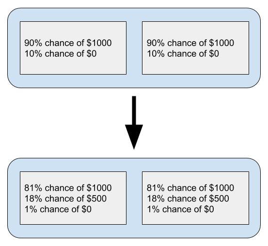
Now put these two together, and split the pool into two new bets, each an average of the original two:

CDOs 2

Take a look at what we’ve obtained. Now we have only a 1% chance of getting nothing (because both bets have to fail for this to happen). We do, however, have only a 81% chance of getting $1000, as opposed to the 90% we had earlier. But what about risk? Are we higher or lower risk than before?

The usual way of measuring risk is to look at standard deviations. So what are the standard deviations of the original bet and the new one?

Initial Bet
Mean = 90% ($1000) + 10% ($0) = $900
Variance = 90% (100^2) + 10% (900^2) = 90,000
Standard deviation = $300

New Bet
Mean = 81% ($1000) + 18% ($500) + 10% ($0) = $900
Variance = 81% (100^2) + 18% (400^2) + 1% (900^2) = 45,000
Standard deviation = $216.13

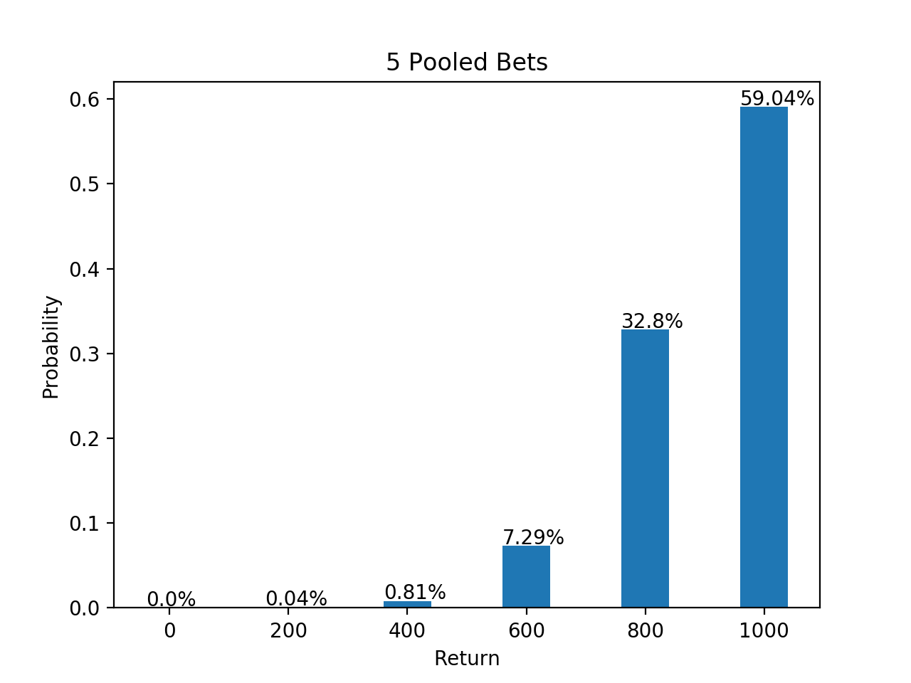
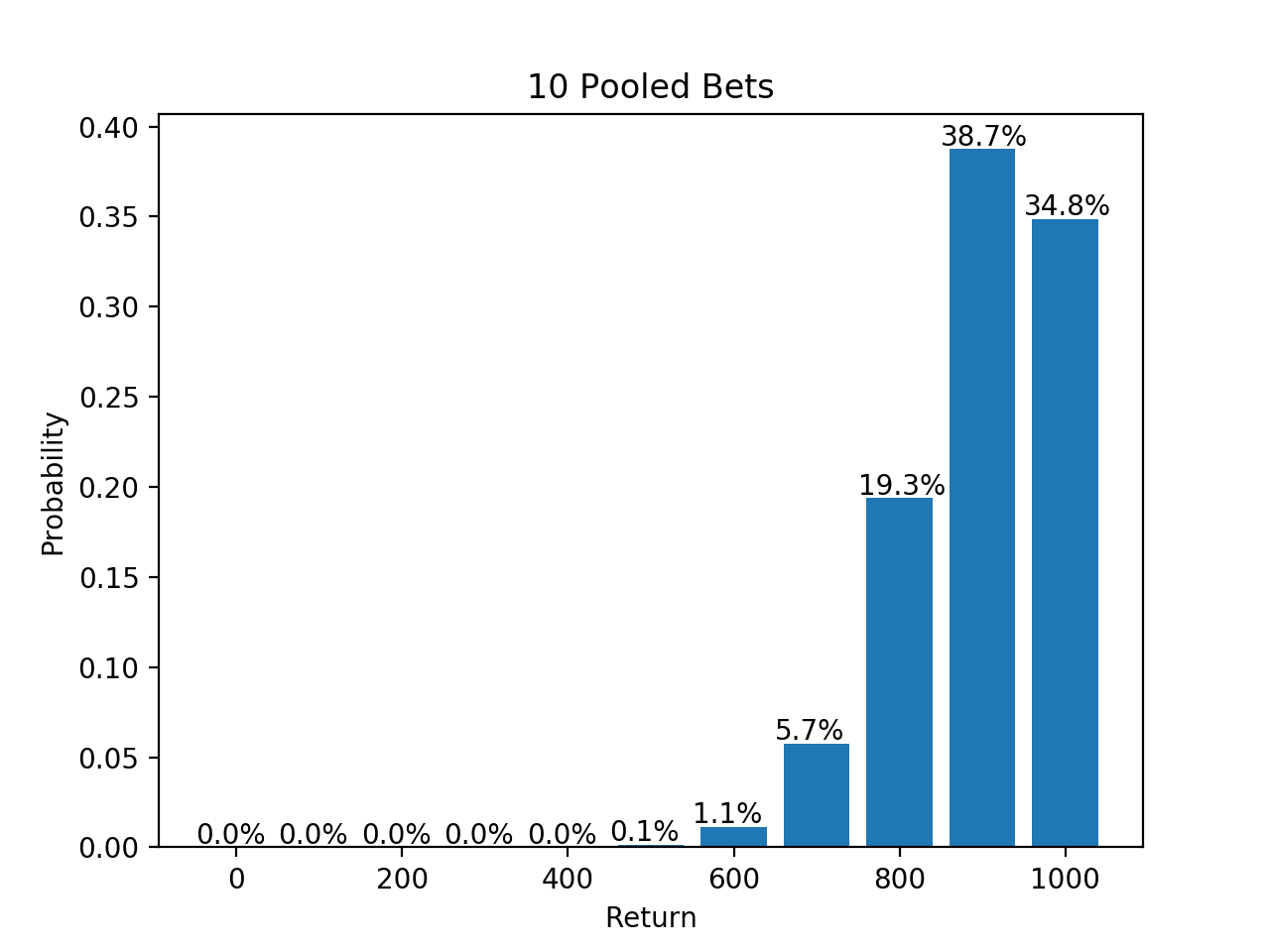
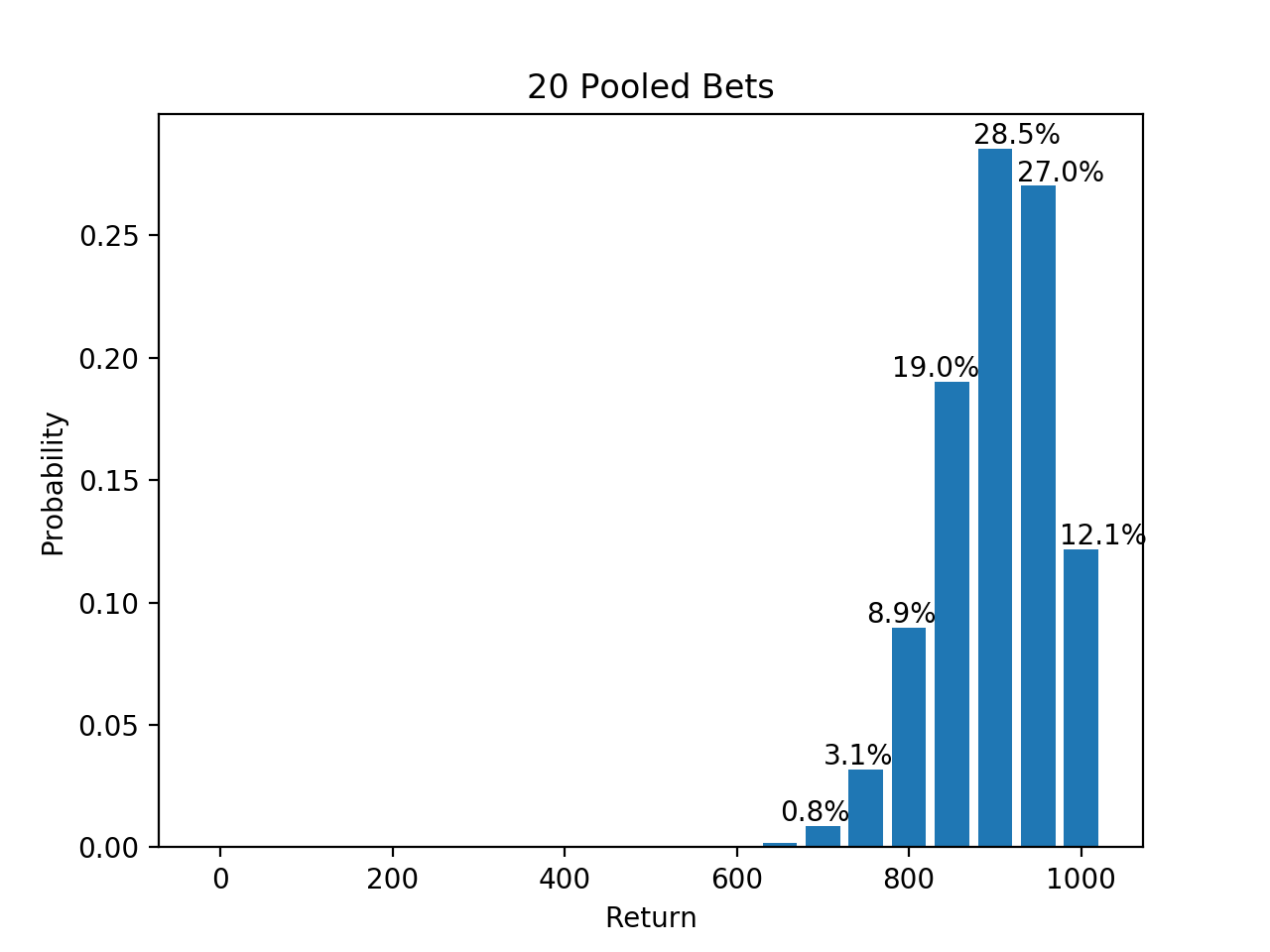
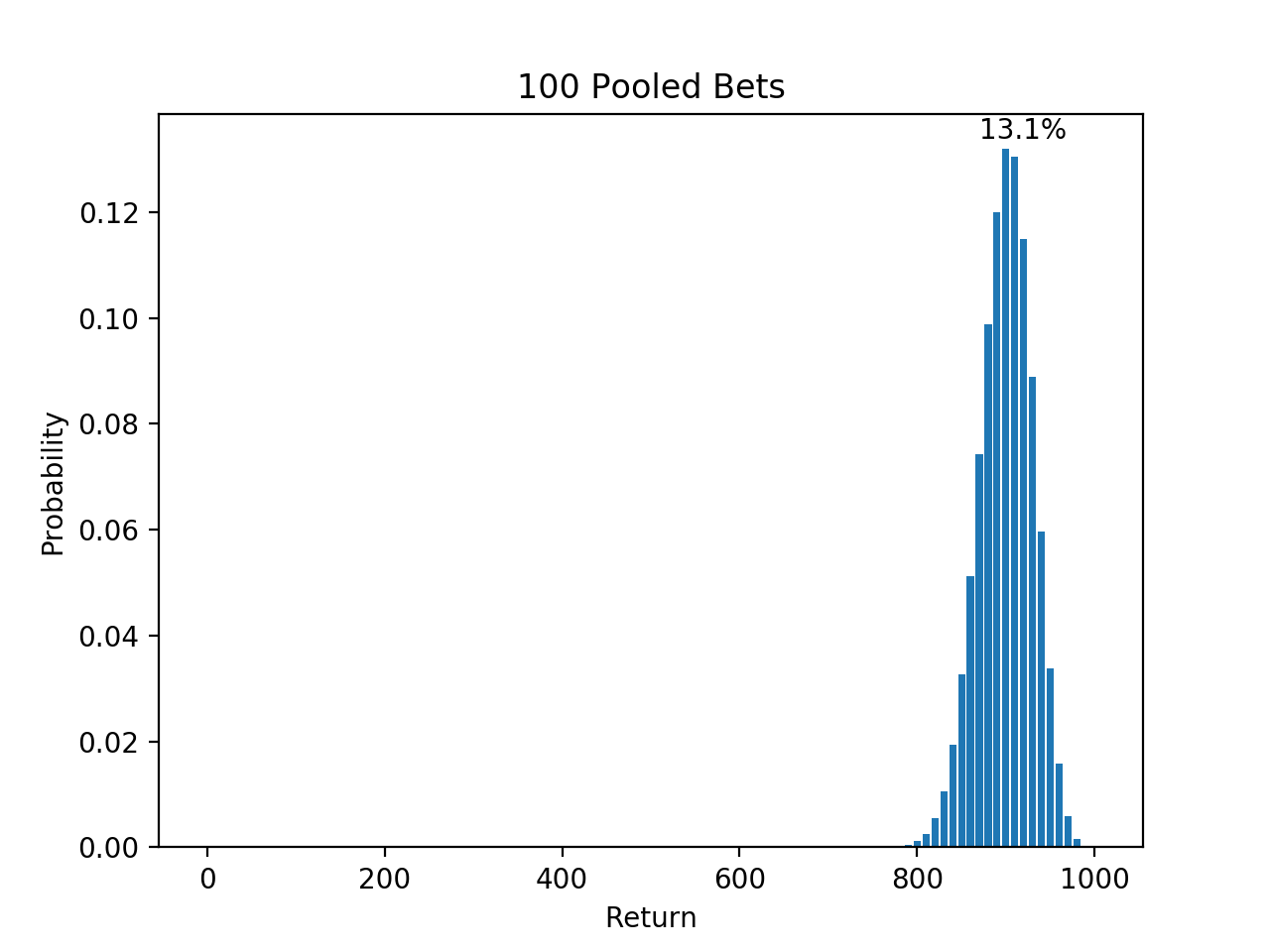
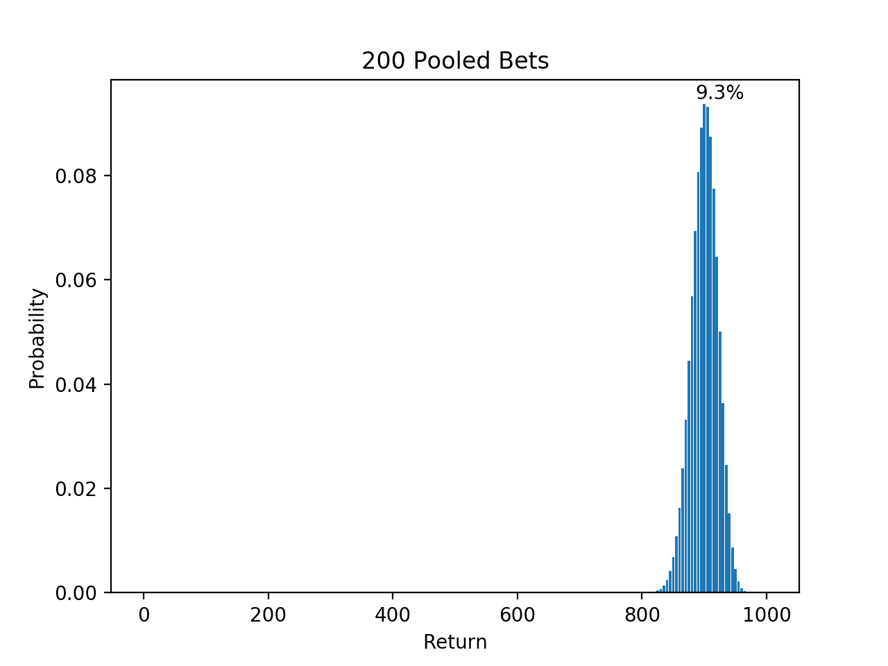
And look at what we see: risk has dropped, and fairly dramatically so, just by pooling independent bets! This concept is one of the core lessons of financial theory, and it goes by the name of diversification. The more bets we pool, the further the risk goes down, and in the limit of infinite independent bets, the risk goes to zero.

5 Pooled Bets10 Pooled Bets20 Pooled Bets100 Pooled Bets200 Pooled Bets

So if you’re watching a movie and somebody says something about combining risky assets to produce safe assets as if that idea is self-evidently absurd, you know that they have no understanding of basic financial concepts, and especially not a complex financial instrument like a CDO.

In fact, let’s move on to CDOs now. The setup I described above of simply pooling bets does decrease risk, but it’s not how CDOs work. At least, not entirely. CDOs still take advantage of diversification, but they also incorporate an additional clever trick to distribute risk.

The idea is that you take a pool of risky assets, and you create from it a new pool of non-identical assets with a spectrum of risk profiles. Previously all of the assets that we generated were identical to each other, but what we’ll do now with the CDO is that we’ll split up our assets into non-identical assets in such a way as to allocate the risk, so that some of the assets that we get will have very high risk (they’ll have more of the risk allocated to them), and some of them will have very little risk.

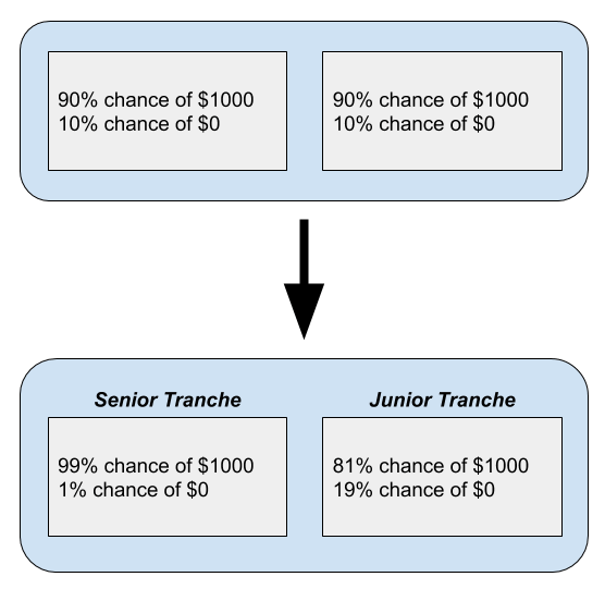
Alright, so that’s the idea: from a pool of equally risky assets, you can get a new pool of assets that have some variation in riskiness. Some of them are actually very safe, and some of them are very, very risky.  How do we do this? Well let’s go back to our starting example where we had two identical bets, each with 90% chance of paying out $1000, and put them together in a pool. But this time, instead of creating two new identical bets, we are going to differentiate the two bets by placing an order priority of payout on them. In other words, one bet will be called the “senior tranche”, and will be paid first. And the other bet will be called the “junior tranche”, and will be paid only if there is still money left over after the senior tranche has been paid. What do the payouts for these two new bets look like?

CDOs (1)

The senior tranche gets paid as long as at least one of the two bets pays out, which happens with 99% probability. Remember, we started with only a 90% probability of paying out. This is a dramatic change! In terms of standard deviation, this is $99.49, less than a third of what we started with!

And what about the junior tranche? Its probability of getting paid is just the probability that both people don’t default, which is 81%. And its risk has gone up, with a standard deviation of $392.30. So essentially, all we’ve done is split up our risk. We originally had 90%/90%, and now we have 99%/81%. In the process, what we’ve done is we’ve created a very very safe bet and a very very risky bet.

Standard Deviations
Original: $300
Simple pooling: $216.13
CDO senior tranche: $99.49
CDO junior tranche: $392.30

The important thing is that these two bets have to both be sold. You can’t just sell the senior tranche to people who want safe things (pension funds), you have to also sell the junior tranche. So how do you do that? Well, you just lower its price! A higher rate of return awaits the taker of the junior tranche in exchange for taking on more risk.

Now if you think about it, this new lower level risk we’ve obtained, this 1% chance of defaulting that we got out of two bets that had a 10% chance of defaulting each, that’s a real thing! There really is a 1% chance that both bets default if they are independent, and so the senior tranche really can expect to get paid 99% of the time! There isn’t a lie or a con here, a pension funds that gets sold these senior tranches of CDOs is actually getting a safe bet! It’s just a clever way of divvying up risk among two assets.

I think the idea of a CDO is cool enough by itself, but I think that the especially cool thing about CDOs is that they open up the market to new customers. Previously, if you wanted to get a mortgage, then you had to find basically a bank that was willing to accept your level of risk, whatever it happens to be. And it could be that if you’re too high risk, then nobody wants to give you a mortgage, and you’d just be out of luck. Even prior to CDOs, when you had mortgage pooling but no payment priority, you have to have investors that are interested in the level of risk of your pool. The novelty of CDOS is in allowing you to alter the risk profile of your pool of mortgages at will.

:Let’s say that you have 100 risky loans, and there’s only enough demand for you to sell 50 of them. What you can do is create a CDO with 50 safe loans and 50 risky loans. Now you get to not only sell your risky loans, but you can also sell your safe loans to interested customers like pension funds! This is the primary benefit of the new financial technology of CDOs: it allows banks to generate tailor-made risk levels for the set of investors that are interested in buying, so that they can sell more mortgage-backed securities and get more people homes. And if everything is done exactly as I described it, then everything should work out fine.

But of course, things weren’t done exactly as I described them. The risk levels of individual mortgages were given increasingly optimistic ratings with stated-income loans, no-down-payment loans, and no-income no-asset loans. CDOs were complex and their risk level was often difficult to assess, resulting in less transparency and more ability for banks to over-report their safety. And crucially, the different tranches of any given CDO are highly dependent on each other, even after they’ve been sold to investors that have nothing to do with each other.

Let’s go back to our simple example of the two $1000 bets for illustration. Suppose that one of the two bets doesn’t pay out (which could correspond to one home-owner defaulting on their monthly payment). Now the senior tranche owner’s payment is entirely dependent on how the other bet performs. The senior tranche owner will get $1000 only if that remaining bet pays out, which happens with just 90% probability. So his chance of getting $1000 has dropped from 99% to 90%.

CDOs 4

That’s a simple example of a more general point: that in a CDO, once the riskier tranches fail, the originally safe tranches suddenly become a lot riskier (so that what was originally AA is now maybe BBB). This helps to explain why once the housing bubble had popped, all levels of CDOs began losing value, not just the junior levels. Ordinary mortgage backed securities don’t behave this way! A AA-rated mortgage is rated that way because of some actual underlying fact about the reliability of the homeowner, which doesn’t necessarily change when less reliable homeowners start defaulting. A AA-rated CDO tranche might be rated that way entirely because it has payment priority, even though all the mortgages in its pool are risky.

Another way to say this: An ordinary mortgage backed security decreased risk just because of diversification (many mortgages pooled together make for a less risky bet than a single mortgage). But a CDO gets decreased risk because of both diversification and (in the upper tranches) the order priority (getting paid first). In both cases, as some of the mortgages in the pool fail, you lose some of the diversification benefit. But in the CDO case, you also lose the order priority benefit in the upper tranches (because, for example, if it takes 75 defaults in your pool for you to lose your money and 50 have already failed, then you are at a much higher risk of losing your money than if none of them have failed). Thus there is more loss of value in safe CDOs than in safe MBSs as default rates rise.

The Central Paradox of Statistical Mechanics: The Problem of The Past

This is the third part in a three-part series on the foundations of statistical mechanics.

  1. The Necessity of Statistical Mechanics for Getting Macro From Micro
  2. Is The Fundamental Postulate of Statistical Mechanics A Priori?
  3. The Central Paradox of Statistical Mechanics: The Problem of The Past

— — —

What I’ve argued for so far is the following set of claims:

  1. To successfully predict the behavior of macroscopic systems, we need something above and beyond the microphysical laws.
  2. This extra thing we need is the fundamental postulate of statistical mechanics, which assigns a uniform distribution over the region of phase space consistent with what you know about the system. This postulate allows us to prove all the things we want to say about the future, such as “gases expand”, “ice cubes melt”, “people age” and so on.
  3. This fundamental postulate is not justifiable on a priori grounds, as it is fundamentally an empirical claim about how frequently different micro states pop up in our universe. Different initial conditions give rise to different such frequencies, so that a claim to a priori access to the fundamental postulate is a claim to a priori access to the precise details of the initial condition of the universe.

 There’s just one problem with all this… apply our postulate to the past, and everything breaks.

 Notice that I said that the fundamental postulate allows us to prove all the things we want to say about the future. That wording was chosen carefully. What happens if you try to apply the microphysical laws + the fundamental postulate to predict the past of some macroscopic system? It turns out that all hell breaks loose. Gases spontaneously contract, ice cubes form from puddles of water, and brains pop out of thermal equilibrium.

 Why does this happen? Very simply, we start with two fully time reversible premises (the microphysical laws and the fundamental postulate). We apply it to present knowledge of some state, the description of which does not specify a special time direction. So any conclusion we get must as a matter of logic be time reversible as well! You can’t start with premises that treat the past as the mirror image of the future, and using just the rules of logical equivalence derive a conclusion that treats the past as fundamentally different from the future. And what this means is that if you conclude that entropy increases towards the future, then you must also conclude that entropy increases towards the past. Which is to say that we came from a higher entropy state, and ultimately (over a long enough time scale and insofar as you think that our universe is headed to thermal equilibrium) from thermal equilibrium.

Let’s flesh this argument out a little more. Consider a half-melted ice cube sitting in the sun. The microphysical laws + the fundamental postulate tell us that the region of phase space consisting of states in which the ice cube is entirely melted is much much much larger than the region of phase space in which it is fully unmelted. So much larger, in fact, that it’s hard to express using ordinary English words. This is why we conclude that any trajectory through phase space that passes through the present state of the system (the half-melted cube) is almost certainly going to quickly move towards the regions of phase space in which the cube is fully melted. But for the exact same reason, if we look at the set of trajectories that pass through the present state of the system, the vast vast vast majority of them will have come from the fully-melted regions of phase space. And what this means is that the inevitable result of our calculation of the ice cube’s history will be that a few moments ago it was a puddle of water, and then it spontaneously solidified and formed into a half-melted ice cube.

This argument generalizes! What’s the most likely past history of you, according to statistical mechanics? It’s not that the solar system coalesced from a haze of gases strewn through space by a past supernova, such that a planet would form in the Goldilocks zone and develop life, which would then gradually evolve through natural selection to the point where you are sitting in whatever room you’re sitting in reading this post. This trajectory through phase space is enormously unlikely. The much much much more likely past trajectory of you through phase space is that a little while ago you were a bunch of particles dispersed through a universe at thermal equilibrium, which happened to spontaneously coalesce into a brain that has time to register a few moments of experience before dissipating back into chaos. “What about all of my memories of the past?” you say. As it happens the most likely explanation of these memories is not that they are veridical copies of real happenings in the universe but illusions, manufactured from randomness.

Basically, if you buy everything I’ve argued in the first two parts, then you are forced to conclude that the universe is most likely near thermal equilibrium, with your current experience of it arising as a spontaneous dip in entropy, just enough to produce a conscious brain but no more. There are at least two big problems with this view.

Problem 1: This conclusion is, we think, extremely empirically wrong! The ice cube in front of you didn’t spontaneously form from a puddle of water, uncracked eggs weren’t a moment ago scrambled, and your memories are to some degree veridical. If you really believe that you are merely a spontaneous dip in entropy, then your prediction for the next minute will be the gradual dissolution of your brain and loss of consciousness. Now, wait a minute and see if this happens. Still here? Good!

Problem 2: The conclusion cannot be simultaneously believed and justified. If you think that you’re a thermal fluctuation, then you shouldn’t credit any of your memories as telling you anything about the world. But then your whole justification to coming to the conclusion in the first place (the experiments that led us to conclude that physics is time-reversible and that the fundamental postulate is true) is undermined! Either you believe it without justification, or you don’t believe despite justification. Said another way, no reflective equilibrium exists at an entropy minimum. David Albert calls this peculiar epistemic state cognitively unstable, as it’s not clear where exactly it should leave you.

Reflect for a moment on how strange of a situation we are in here. Starting from very basic observations of the world, involving its time-reversibility on the micro scale and the increase in entropy of systems, we see that we are inevitably led to the conclusion that we are almost certainly thermal fluctuations, brains popping out of the void. I promise you that no trick has been pulled here, this really is the state of the philosophy of statistical mechanics! The big issue is how to deal with this strange situation.

One approach is to say the following: Our problem is that our predictions work towards the future but not the past. So suppose that we simply add as a new fundamental postulate the proposition that long long ago the universe had an incredibly low entropy. That is, suppose that instead of just starting with the microphysical laws and the fundamental postulate of statistical mechanics, we added a third claims: the Past Hypothesis.

The Past Hypothesis should be understood as an augmentation of our Fundamental Postulate. Taken together, the two postulates say that our probability distribution over possible microstates should not be uniform over phase space. Instead, it should be what you get when you take the uniform distribution, and then condition on the distant past being extremely low entropy. This process of conditioning clearly preferences one direction of time over the other, and so the symmetry is broken.

 It’s worth reflecting for a moment on the strangeness of the epistemic status of the Past Hypothesis. It happens that we have over time accumulated a ton of observational evidence for the occurrence of the Big Bang. But none of this evidence has anything to do with our reasons for accepting the Past Hypothesis. If we buy the whole line of argument so far, our conclusion that something like a Big Bang occurred becomes something that we are forced to believe for deep logical reasons, on pain of cognitive instability and self-undermining belief. Anybody that denies that the Big Bang (or some similar enormously low-entropy past state) occurred has to contend with their view collapsing in self-contradiction upon observing the physical laws!

Is The Fundamental Postulate of Statistical Mechanics A Priori?

This is the second part in a three-part series on the foundations of statistical mechanics.

  1. The Necessity of Statistical Mechanics for Getting Macro From Micro
  2. Is The Fundamental Postulate of Statistical Mechanics A Priori?
  3. The Central Paradox of Statistical Mechanics: The Problem of The Past

— — —

The fantastic empirical success of the fundamental postulate gives us a great amount of assurance that the postulate is good one. But it’s worth asking whether that’s the only reason that we should like this postulate, or if it has some solid a priori justification. The basic principle of “when you’re unsure, just distribute credences evenly over phase space” certainly strikes many people as highly intuitive and justifiable on a priori grounds. But there are some huge problems with this way of thinking, one of which I’ve already hinted at. Here’s a thought experiment that illustrates the problem.

There is a factory in your town that produces cubic boxes. All you know about this factory is that the boxes that they produce all have a volume between 0 m3 and 1 m3. You are going to be delivered a box produced by this factory, and are asked to represent your state of knowledge about the box with a probability distribution. What distribution should you use?

Suppose you say “I should be indifferent over all the possible boxes. So I should have a uniform distribution over the volumes from 0 m3 to 1 m3.” This might seem reasonable at first blush. But what if somebody else said “Yes, you should be indifferent over all the possible boxes, but actually the uniform distribution should be over the side lengths from 0 m to 1 m, not volumes.” This would be a very different probability distribution! For example, if the probability that the side length is greater than .5 m is 50%, then the probability that the volume is greater than (.5)3 = 1/8 is also 50%! Uniform over side length is not the same as uniform over volume (or surface area, for that matter). Now, how do you choose between a uniform distribution over volumes and a uniform distribution over side lengths? After all, you know nothing about the process that the factory is using to produce the boxes, and whether it is based off of volume or side length (or something else); all you know is that all boxes are between 0 m3 and 1 m3.

The lesson of this thought experiment is that the statement we started with (“I should be indifferent over all possible boxes”) was actually not even well-defined. There’s not just one unique measure over a continuous space, and in general the notion that “all possibilities are equally likely” is highly language-dependent.

The exact same applies to phase space, as position and momentum are continuous quantities. Imagine that somebody instead of talking about phase space, only talked about “craze space”, in which all positions become positions cubed, and all momentum values become natural logs of momentum. This space would still contain all possible microstates of your system. What’s more, the fundamental laws of nature could be rewritten in a way that uses only craze space quantities, not phase space quantities. And needless to say, being indifferent over phase space would not be the same as being indifferent over craze space.

Spend enough time looking at attempts to justify a unique interpretation of the statement “All states are equally likely”, when your space of states is a continuous infinity, and you’ll realize that all such attempts are deeply dependent upon arbitrary choices of language. The maximum information entropy probability distribution is afflicted with the exact same problem, because the entropy of your distribution is going to depend on the language you’re using to describe it! The entropy of a distribution in phase space is NOT the same as the entropy of the equivalent distribution transformed to craze space.

Let’s summarize this section. If somebody tells you that the fundamental postulate says that all microstates compatible with what you know about the macroscopic features of your system are equally likely, the proper response is something like “Equally likely? That sounds like you’re talking about a uniform distribution. But uniform over what? Oh, position and momentum? Well, why’d you make that choice?” And if they point out that the laws of physics are expressed in terms of position and momentum, you just disagree and say “No, actually I prefer writing the laws of physics in terms of position cubed and log momentum!” (Substitute in any choice of monotonic functions).

If they object on the grounds of simplicity, point out that position and momentum are only simple as measured from a standpoint that takes them to be the fundamental concepts, and that from your perspective, getting position and momentum requires applying complicated inverse transformations to your monotonic transformation of the chosen coordinates.

And if they object on the grounds of naturalness, the right response is probably something like “Tell me more about this ’naturalness’. How do you know what’s natural or unnatural? It seems to me that your choice of what physical concepts count as natural is a manifestation of deep selection pressures that push any beings whose survival depends on modeling and manipulating their surroundings towards forming an empirically accurate model of the macroscopic world. So that when you say that position is more natural than log(position), what I hear is that the fundamental postulate is a very useful tool. And you can’t use the naturalness of the choice of position to justify the fundamental postulate, when your perception of the naturalness of position is the result of the empirical success of the fundamental postulate!”

In my judgement, none of the a priori arguments work, and fundamentally the reason is that the fundamental postulate is an empirical claim. There’s no a priori principle of rationality that tells us that boxes of gases tend to equilibrate, because you can construct a universe whose initial microstate is such that its entire history is one of entropy radically decreasing, gases concentrating, eggs unscrambling, ice cubes unmelting, and so on. Why is this possible? Because it’s consistent with the microphysical laws that the universe started in an enormously low entropy configuration, so it’s gotta also be consistent with the microphysical laws for the entire universe to spend its entire lifetime decreasing in entropy. The general principle is: If you believe that something is physically possible, then you should believe its time-inverse is possible as well.

Let’s pause and take stock. What I’ve argued for so far is the following set of claims:

  1. To successfully predict the behavior of macroscopic systems, we need something above and beyond the microphysical laws.
  2. This extra thing we need is the fundamental postulate of statistical mechanics, which assigns a uniform distribution over the region of phase space consistent with what you know about the system. This postulate allows us to prove all the things we want to say about the future, such as “gases expand”, “ice cubes melt”, “people age” and so on.
  3. This fundamental postulate is not justifiable on a priori grounds, as it is fundamentally an empirical claim about how frequently different microstates pop up in our universe. Different initial conditions give rise to different such frequencies, so that a claim to a priori access to the fundamental postulate is a claim to a priori access to the precise details of the initial condition of the universe.

There’s just one problem with all this… apply our postulate to the past, and everything breaks.

Up next: Why does statistical mechanics give crazy answers about the past? Where did we go wrong?

The Necessity of Statistical Mechanics for Getting Macro From Micro

This is the first part in a three-part series on the foundations of statistical mechanics.

  1. The Necessity of Statistical Mechanics for Getting Macro From Micro
  2. Is The Fundamental Postulate of Statistical Mechanics A Priori?
  3. The Central Paradox of Statistical Mechanics: The Problem of The Past

— — —

Let’s start this out with a thought experiment. Imagine that you have access to the exact fundamental laws of physics. Suppose further that you have unlimited computing power, for instance, you have an oracle that can instantly complete any computable task. What then do you know about the world?

The tempting answer: Everything! But of course, upon further consideration, you are missing a crucial ingredient: the initial conditions of the universe. The laws themselves aren’t enough to tell you about your universe, as many different universes are compatible with the laws. By specifying the state of the universe at any one time (which incidentally does not have to be an “initial” time), though, you should be able to narrow down this set of compatible universes. So let’s amend our question:

Suppose that you have unlimited computing power, that you know the exact microphysical laws, and that you know the state of the universe at some moment. Then what do you know about the world?

The answer is: It depends! What exactly do you know about the state of the universe? Do you know it’s exact microstate? As in, do you know the position and momentum of every single particle in the universe? If so, then yes, the entire past and future of the universe are accessible to you. But suppose that instead of knowing the exact microstate, you only have access to a macroscopic description of the universe. For example, maybe you have a temperature map as well as a particle density function over the universe. Or perhaps you know the exact states of some particles, just not all of them.

Well, if you only have access to the macrostate of the system (which, notice, is the epistemic situation that we find ourselves in, being that full access to the exact microstate of the universe is as technologically remote as can be), then it should be clear that you can’t specify the exact microstate at all other times. This is nothing too surprising or interesting… starting with imperfect knowledge you will not arrive at perfect knowledge. But we might hope that in the absence of a full description of the microstate of the universe at all other times, you could at least give a detailed macroscopic description of the universe at other times.

That is, here’s what seems like a reasonable expectation: If I had infinite computational power, knew the exact microphysical laws, and knew, say, that a closed box was occupied by a cloud of noninteracting gas in its corner, then I should be able to draw the conclusion that “The gas will disperse.” Or, if I knew that an ice cube was sitting outdoors on a table in the sun, then I should be able to apply my knowledge of microphysics to conclude that “The ice cube will melt”. And we’d hope that in addition to being able to make statements like these, we’d also be able to produce precise predictions for how long it would take for the gas to become uniformly distributed over the box, or for how long it would take for the ice cube to melt.

Here is the interesting and surprising bit. It turns out that this is in principle impossible to do. Just the exact microphysical laws and an infinity of computing power is not enough to do the job! In fact, the microphysical laws will in general tell us almost nothing about the future evolution or past history of macroscopic systems!

Take this in for a moment. You might not believe me (especially if you’re a physicist). For one thing, we don’t know the exact form of the microphysical laws. It would seem that such a bold statement about their insufficiencies would require us to at least first know what they are, right? No, it turns out that the statement that microphysics is is far too weak to tell us about the behavior of macroscopic systems holds for an enormously large class of possible laws of physics, a class that we are very sure that our universe belongs to.

Let’s prove this. We start out with the following observation that will be familiar to physicists: the microphysical laws appear to be time-reversible. That is, it appears to be the case that for every possible evolution of a system compatible with the laws of physics, the time-reverse of that evolution (obtained by simply reversing the trajectories of all particles) is also perfectly compatible with the laws of physics.*

This is surprising! Doesn’t it seem like there are trajectories that are physically possible for particles to take, such that their time reverse is physically impossible? Doesn’t it seem like classical mechanics would say that a ball sitting on the ground couldn’t suddenly bounce up to your hand? An egg unscramble? A gas collect in the corner of a room? The answer to all of the above is no. Classical mechanics, and fundamental physics in general, admits the possibilities of all these things. A fun puzzle for you is to think about why the first example (the ball initially at rest on the ground bouncing up higher and higher until it comes to rest in your hand) is not a violation of the conservation of energy.

Now here’s the argument: Suppose that you have a box that you know is filled with an ideal gas at equilibrium (uniformly spread through the volume). There are many many (infinitely many) microstates that are compatible with this description. We can conclusively say that in 15 minutes the gas will still be dispersed only if all of these microstates, when evolved forward 15 minutes, end up dispersed.

But, and here’s the crucial step, we also know that there exist very peculiar states (such as the macrostate in which all the gas particles have come together to form a perfect statuette of Michael Jackson) such that these states will in 15 minutes evolve to the dispersed state. And by time reversibility, this tells us that there is another perfectly valid history of the gas that starts uniformly dispersed and evolves over 15 minutes into a perfect statuette of Michael Jackson. That is, if we believe that complicated configurations of gases disperse, and believe that physics is time-reversible, then you must also believe that there are microstates compatible with dispersed states of gas that will in the next moment coalesce into some complicated configuration.

  1. A collection of gas shaped exactly like Michael Jackson will disperse uniformly across its container.
  2. Physics is time reversible.
  3. So uniformly dispersed gases can coalesce into a collection of gases shaped exactly like Michael Jackson.

At this point you might be thinking “yeah, sure, microphysics doesn’t in principle rule out the possibility that a uniformly dispersed gas will coalesce into Michael Jackson, or any other crazy configuration. But who cares? It’s so incredibly unlikely!” To which the response is: Yes, exactly, it’s extremely unlikely. But nothing in the microphysical laws says this! Look as hard as you can at the laws of motion, you will not find a probability distribution over the likelihood of the different microstates compatible with a given macrostate. And indeed, different initial conditions of the universe will give different such frequencies distributions! To make any statements about the relative likelihood of some microstates over others, you need some principle above and beyond the microphysical laws.

To summarize. All that microphysics + infinite computing power allows you to say about a macrostate is the following: Here are all the microstates that are compatible with that macrostate, and here are all the past and future histories of each of these microstates. And given time reversibility, these future histories cover an enormously diverse set of predictions about the future, from “the gas will disperse” to “the gas will form into a statuette of Michael Jackson”. To get reasonable predictions about how the world will actually behave, we need some other principle, a principle that allows us to disregard these “perverse” microstates. And microphysics contains no such principle.

Statistical mechanics is thus the study of the necessary augmentation to a fundamental theory of physics that allows us to make predictions about the world, given that we are not in the position to know its exact microstate. This necessary augmentation is known as the fundamental postulate of statistical mechanics, and it takes the form of a probability distribution over microstates. Some people describe the postulate as saying “all microstates being equally likely”, but that phrasing is a big mistake, as the sentence “all states are equally likely” is not well defined over a continuous set of states. (More on that in a bit.) To really understand the fundamental postulate, we have to introduce the notion of phase space.

The phase space for a system is a mathematical space in which every point represents a full specification of the positions and momenta of all particles in the system. So, for example, a system consisting of 1000 classical particles swimming around in an infinite universe would have 6000 degrees of freedom (three position coordinates and three momentum coordinates per particle). Each of these degrees of freedom is isomorphic to the real numbers. So phase space for this system must be 6000, and a point in phase space is a specification of the values of all 6000 degrees of freedom. In general, for N classical particles, phase space is 6N.

With the concept of phase space in hand, we can define the fundamental postulate of statistical mechanics. This is: the probability distribution over microstates compatible with a given macrostate is uniform over the corresponding volume of phase space.

It turns out that if you just measure the volume of the “perverse states” in phase space, you end up finding that it composes approximately 0% of the volume of compatible microstates in phase space. This of course allows us to say of perverse states, “Sure they’re there, and technically it’s possible that my system is in such a state, but it’s so incredibly unlikely that it makes virtually no impact on my prediction of the future behavior of my system.” And indeed, when you start going through the math and seeing the way that systems most likely evolve given the fundamental postulate, you see that the predictions you get match beautifully with our observations of nature.

Next time: What is the epistemic status of the fundamental postulate? Do we have good a priori reasons to believe it?

— — —

* There are some subtleties here. For one, we think that there actually is a very small time asymmetry in the weak nuclear force. And some collapse interpretations of quantum mechanics have the collapse of the wave function as an irreversible process, although Everettian quantum mechanics denies this. For the moment, let’s disregard all of that. The time asymmetry in the weak nuclear force is not going to have any relevant effect on the proof made here, besides making it uglier and more complicated. What we need is technically not exact time-reversibility, but very-approximate time-reversibility. And that we have. Collapsing wave functions are a more troubling business, and are a genuine way out of the argument made in this post.

A Cognitive Instability Puzzle, Part 2

This is a follow of this previous post, in which I present three unusual cases of belief updating. Read it before you read this.

I find these cases very puzzling, and I don’t have a definite conclusion for any of them. They share some deep similarities. Let’s break all of them down into their basic logical structure:

Joe
Joe initially believes in classical logic and is certain of some other stuff, call it X.
An argument A exists that concludes that X can’t be true if classical logic is true.
If Joe believes classical logic, then he believes A.
If Joe believes intuitionist logic, then he doesn’t believe A.

Karl
Karl initially believes in God and is certain of some other stuff about evil, call it E.
An argument A exists that concludes that God can’t exist if E is true.
If Karl believes in God, then he believes A.
If Karl doesn’t believe in God, then he doesn’t believe A.

Tommy
Tommy initially believes in her brain’s reliability and is certain of some other stuff about her experiences, call it Q.
An argument A exists that concludes that hat her brain can’t be reliable if Q is true.
If Tommy believes in her brain’s reliability, then she believes A.
If Tommy doesn’t believe in her brain’s reliability, then she doesn’t believe A.

First of all, note that all three of these cases are ones in which Bayesian reasoning won’t work. Joe is uncertain about the law of the excluded middle, without which you don’t have probability theory. Karl is uncertain about the meaning of the term ‘evil’, such that the same proposition switches from being truth-apt to being meaningless when he updates his beliefs. Probability theory doesn’t accommodate such variability in its language. And Tommy is entertaining a hypothesis according to which she no longer accepts any deductive or inductive logic, which is inconsistent with Bayesianism in an even more extreme way than Joe.

The more important general theme is that in all three cases, the following two things are true: 1) If an agent believes A, then they also believe an argument that concludes -A. 2) If that agent believes -A, then they don’t believe the argument that concludes -A.

Notice that if an agent initially doesn’t believe A, then they have no problem. They believe -A, and also happen to not believe that specific argument concluding -A, and that’s fine! There’s no instability or self-contradiction there whatsoever. So that’s really not where the issue lies.

The mystery is the following: If the only reason that an agent changed their mind from A to -A is the argument that they no longer buy, then what should they do? Once they’ve adopted the stance that A is false, should they stay there, reasoning that if they accept A they will be led to a contradiction? Or should they jump back to A, reasoning that the initial argument that led them there was flawed?

Said another way, should they evaluate the argument against A from their own standards, or from A’s standards? If they use their own standards, then they are in an unstable position, where they jump back and forth between A and -A. And if they always use A’s standards… well, then we get the conclusion that Tommy should believe herself to be a Boltzmann brain. In addition, if they are asked why they don’t believe A, then they find themselves in the weird position of giving an explanation in terms of an argument that they believe to be false!

I find myself believing that either Joe should be an intuitionist, Karl an atheist, and Tommy a radical skeptic, OR Joe a classical-logician, Karl a theist, and Tommy a reliability-of-brain-believer-in. That is, it seems like there aren’t any significant enough disanalogies between these three cases to warrant concluding one thing in one case and then going the other direction in another.

Hopping Midpoints

Put down three points on a piece of paper. Choose one of them as your “starting point”. Now, randomly choose one of the three points and hop from your starting point, halfway over to the chosen point. Mark down where you’ve landed. Then repeat: randomly choose one of the three starting points, and move halfway from your newly marked point to this new chosen point. Mark where you land. And on, and on, to infinity.

What pattern will arise? Watch and see!

Controls:
E to increase points/second.
Q to decrease points/second.
Click and drag the red points to move them around.
Pressing a number key will make a polygon with that number of sides.
[pjs4wp]
float N = 3;
float[] X = new float(N);
float[] Y = new float(N);
float radius = 600/2 – 20;
float i = 0;
while (N > i)
{
X[i] = radius * cos(2*PI*i/N – PI/2 + 2*PI/N);
Y[i] = radius * sin(2*PI*i/N – PI/2 + 2*PI/N);
i += 1;
}
float xNow = X[0];
float yNow = Y[0];
float speed = 1;
int selected = -1;
void setup()
{
size(600,600);
frameRate(10);
background(0);
}
void draw()
{
fill(255);
stroke(255);
text((str)(speed*10) + ” points / second\nE to speed up\nQ to slow down\nClick and drag red points!”,15,25);
translate(width/2, height/2);
float i = 0;
while(i < speed) { point(xNow, yNow); index = (int)(random(N)); xNow = (xNow + X[index])/2; yNow = (yNow + Y[index])/2; i += 1; } stroke(color(255,0,0)); fill(color(255,0,0)); float j = 0; while (N > j)
{
ellipse(X[j],Y[j],10,10);
j += 1;
}
}
void keyReleased()
{
bool reset = 0;
if (key == ‘e’) speed *= 10;
else if (key == ‘q’ && speed > 1) speed /= 10;
else if (key == ‘2’) N = 2;
else if (key == ‘3’) N = 3;
else if (key == ‘4’) N = 4;
else if (key == ‘5’) N = 5;
else if (key == ‘6’) N = 6;
else if (key == ‘7’) N = 7;
else if (key == ‘8’) N = 8;
else if (key == ‘9’) N = 9;
else reset = 1;
if (reset == 0)
{
background(0);
float i = 0;
while (N > i)
{
X[i] = radius * cos(2*PI*i/N – PI/2);
Y[i] = radius * sin(2*PI*i/N – PI/2);
i += 1;
}
xNow = X[0];
yNow = Y[0];
}
}
void mousePressed()
{
if (selected == -1)
{
float i = 0;
while (N > i)
{
if ((X[i] + 5 >= mouseX – width/2) && (mouseX – width/2 >= X[i] – 5))
if ((Y[i] + 5 >= mouseY – height/2) && (mouseY – height/2 >= Y[i] – 5))
selected = i;
i += 1;
}
}
}
void mouseReleased()
{
if (selected != -1)
{
X[selected] = mouseX – width/2;
Y[selected] = mouseY – height/2;
selected = -1;
xNow = X[0];
yNow = Y[0];
background(0);
}
}
[/pjs4wp]

The problem with the many worlds interpretation of quantum mechanics

The Schrodinger equation is the formula that describes the dynamics of quantum systems – how small stuff behaves.

One fundamental feature of quantum mechanics that differentiates it from classical mechanics is the existence of something called superposition. In the same way that a particle can be in the state of “being at position A” and could also be in the state of “being at position B”, there’s a weird additional possibility that the particle is in the state of “being in a superposition of being at position A and being at position B”. It’s necessary to introduce a new word for this type of state, since it’s not quite like anything we are used to thinking about.

Now, people often talk about a particle in a superposition of states as being in both states at once, but this is not technically correct. The behavior of a particle in a superposition of positions is not the behavior you’d expect from a particle that was at both positions at once. Suppose you sent a stream of small particles towards each position and looked to see if either one was deflected by the presence of a particle at that location. You would always find that exactly one of the streams was deflected. Never would you observe the particle having been in both positions, deflecting both streams.

But it’s also just as wrong to say that the particle is in either one state or the other. Again, particles simply do not behave this way. Throw a bunch of electrons, one at a time, through a pair of thin slits in a wall and see how they spread out when they hit a screen on the other side. What you’ll get is a pattern that is totally inconsistent with the image of the electrons always being either at one location or the other. Instead, the pattern you’d get only makes sense under the assumption that the particle traveled through both slits and then interfered with itself.

If a superposition of A and B is not the same as “A and B’ and it’s not the same as ‘A or B’, then what is it? Well, it’s just that: a superposition! A superposition is something fundamentally new, with some of the features of “and” and some of the features of “or”. We can do no better than to describe the empirically observed features and then give that cluster of features a name.

Now, quantum mechanics tells us that for any two possible states that a system can be in, there is another state that corresponds to the system being in a superposition of the two. In fact, there’s an infinity of such superpositions, each corresponding to a different weighting of the two states.

The Schrödinger equation is what tells how quantum mechanical systems evolve over time. And since all of nature is just one really big quantum mechanical system, the Schrödinger equation should also tell us how we evolve over time. So what does the Schrödinger equation tell us happens when we take a particle in a superposition of A and B and make a measurement of it?

The answer is clear and unambiguous: The Schrödinger equation tells us that we ourselves enter into a superposition of states, one in which we observe the particle in state A, the other in which we observe it in B. This is a pretty bizarre and radical answer! The first response you might have may be something like “When I observe things, it certainly doesn’t seem like I’m entering into a superposition… I just look at the particle and see it in one state or the other. I never see it in this weird in-between state!”

But this is not a good argument against the conclusion, as it’s exactly what you’d expect by just applying the Schrödinger equation! When you enter into a superposition of “observing A” and “observing B”, neither branch of the superposition observes both A and B. And naturally, since neither branch of the superposition “feels” the other branch, nobody freaks out about being superposed.

But there is a problem here, and it’s a serious one. The problem is the following: Sure, it’s compatible with our experience to say that we enter into superpositions when we make observations. But what predictions does it make? How do we take what the Schrödinger equation says happens to the state of the world and turn it into a falsifiable experimental setup? The answer appears to be that we can’t. At least, not using just the Schrödinger equation on its own. To get out predictions, we need an additional postulate, known as the Born rule.

This postulate says the following: For a system in a superposition, each branch of the superposition has an associated complex number called the amplitude. The probability of observing any particular branch of the superposition upon measurement is simply the square of that branch’s amplitude.

For example: A particle is in a superposition of positions A and B. The amplitude attached to A is 0.8. The amplitude attached to B is 0.4. If we now observe the position of the particle, we will find it to be at either A with probability (.6)2 (i.e. 36%), or B with probability (.8)2 (i.e. 64%).

Simple enough, right? The problem is to figure out where the Born rule comes from and what it even means. The rule appears to be completely necessary to make quantum mechanics a testable theory at all, but it can’t be derived from the Schrödinger equation. And it’s not at all inevitable; it could easily have been that probabilities associated with the amplitude were gotten by taking absolute values rather than squares. Or why not the fourth power of the amplitude? There’s a substantive claim here, that probabilities associate with the square of the amplitudes that go into the Schrödinger equation, that needs to be made sense of. There are a lot of different ways that people have tried to do this, and I’ll list a few of the more prominent ones here.

The Copenhagen Interpretation

(Prepare to be disappointed.) The Copenhagen interpretation, which has historically been the dominant position among working physicists, is that the Born rule is just an additional rule governing the dynamics of quantum mechanical systems. Sometimes systems evolve according to the Schrödinger equation, and sometimes according to the Born rule. When they evolve according to the Schrödinger equation, they split into superpositions endlessly. When they evolve according to the Born rule, they collapse into a single determinate state. What determines when the systems evolve one way or the other? Something measurement something something observation something. There’s no real consensus here, nor even a clear set of well-defined candidate theories.

If you’re familiar with the way that physics works, this idea should send your head spinning. The claim here is that the universe operates according to two fundamentally different laws, and that the dividing line between the two hinges crucially on what we mean by the words “measurement and “observation. Suffice it to say, if this was the right way to understand quantum mechanics, it would go entirely against the spirit of the goal of finding a fundamental theory of physics. In a fundamental theory of physics, macroscopic phenomena like measurements and observations need to be built out of the behavior of lots of tiny things like electrons and quarks, not the other way around. We shouldn’t find ourselves in the position of trying to give a precise definition to these words, debating whether frogs have the capacity to collapse superpositions or if that requires a higher “measuring capacity”, in order to make predictions about the world (as proponents of the Copenhagen interpretation have in fact done!).

The Copenhagen interpretation is not an elegant theory, it’s not a clearly defined theory, and it’s fundamentally at tension with the project of theoretical physics. So why has it been, as I said, the dominant approach over the last century to understanding quantum mechanics? This really comes down to physicists not caring enough about the philosophy behind the physics to notice that the approach they are using is fundamentally flawed. In practice, the Copenhagen interpretation works. It allows somebody working in the lab to quickly assess the results of their experiments and to make predictions about how future experiments will turn out. It gives the right empirical probabilities and is easy to implement, even if the fuzziness in the details can start to make your head hurt if you start to think about it too much. As Jean Bricmont said, “You can’t blame most physicists for following this ‘shut up and calculate’ ethos because it has led to tremendous develop­ments in nuclear physics, atomic physics, solid­ state physics and particle physics.” But the Copenhagen interpretation is not good enough for us. A serious attempt to make sense of quantum mechanics requires something more substantive. So let’s move on.

Objective Collapse Theories

These approaches hinge on the notion that the Schrödinger equation really is the only law at work in the universe, it’s just that we have that equation slightly wrong. Objective collapse theories add slight nonlinearities to the Schrödinger equation so that systems sometimes spread out in superpositions and other times collapse into definite states, all according to one single equation. The most famous of these is the spontaneous collapse theory, according to which quantum systems collapse with a probability that grows with the number of particles in the system.

This approach is nice for several reasons. For one, it gives us the Born rule without requiring a new equation. It makes sense of the Born rule as a fundamental feature of physical reality, and makes precise and empirically testable predictions that can distinguish it from from other interpretations. The drawback? It makes the Schrödinger equation ugly and complicated, and it adds extra parameters that determine how often collapse happens. And as we know, whenever you start adding parameters you run the risk of overfitting your data.

Hidden Variable Theories

These approaches claim that superpositions don’t really exist, they’re just a high-level consequence of the unusual behavior of the stuff at the smallest level of reality.  They deny that the Schrödinger equation is truly fundamental, and say instead that it is a higher-level approximation of an underlying deterministic reality. “Deterministic?! But hasn’t quantum mechanics been shown conclusively to be indeterministic??” Well, not entirely. For a while there was a common sentiment amongst physicists that John Von Neumann and others had proved beyond a doubt that no deterministic theory could make the predictions that quantum mechanics makes. Later subtle mistakes were found in these purported proofs that left a door open for determinism. Today there are well-known fleshed-out hidden variable theories that successfully reproduce the predictions of quantum mechanics, and do so fully deterministically.

The most famous of these is certainly Bohmian mechanics, also called pilot wave theory. Here’s a nice video on it if you’d like to know more, complete with pretty animations. Bohmian mechanics is interesting, appear to work, give us the Born rule, and is probably empirically distinguishable from other theories (at least in principle). A serious issue with it is that it requires nonlocality, which is a challenge to any attempt to make it consistent with special relativity. Locality is such an important and well-understood feature of our reality that this constitutes a major challenge to the approach.

Many-Worlds / Everettian Interpretations

Ok, finally we talk about the approach that is most interesting in my opinion, and get to the title of this post. The Many-Worlds interpretation says, in essence, that we were wrong to ever want more than the Schrödinger equation. This is the only law that governs reality, and it gives us everything we need. Many-Worlders deny that superpositions ever collapse. The result of us performing a measurement on a system in superposition is simply that we end up in superposition, and that’s the whole story!

So superpositions never collapse, they just go deeper into superposition. There’s not just one you, there’s every you, spread across the different branches of the wave function of the universe. All these yous exist beside each other, living out all your possible life histories.

But then where does Many-Worlds get the Born rule from? Well, uh, it’s kind of a mystery. The Born rule isn’t an additional law of physics, because the Schrödinger equation is supposed to be the whole story. It’s not an a priori rule of rationality, because as we said before probabilities could have easily gone as the fourth power of amplitudes, or something else entirely. But if it’s not an a posteriori fact about physics, and also not an a priori knowable principle of rationality, then what is it?

This issue has seemed to me to be more and more important and challenging for Many-Worlds the more I have thought about it. It’s hard to see what exactly the rule is even saying in this interpretation. Say I’m about to make a measurement of a system in a superposition of states A and B. Suppose that I know the amplitude of A is much smaller than the amplitude of B. I need some way to say “I have a strong expectation that I will observe B, but there’s a small chance that I’ll see A.” But according to Many-Worlds, a moment from now both observations will be made. There will be a branch of the superposition in which I observe A, and another branch in which I observe B. So what I appear to need to say is something like “I am much more likely to be the me in the branch that observes B than the me that observes A.” But this is a really strange claim that leads us straight into the thorny philosophical issue of personal identity.

In what sense are we allowed to say that one and only one of the two resulting humans is really going to be you? Don’t both of them have equal claim to being you? They each have your exact memories and life history so far, the only difference is that one observed A and the other B. Maybe we can use anthropic reasoning here? If I enter into a superposition of observing-A and observing-B, then there are now two “me”s, in some sense. But that gives the wrong prediction! Using the self-sampling assumption, we’d just say “Okay, two yous, so there’s a 50% chance of being each one” and be done with it. But obviously not all binary quantum measurements we make have a 50% chance of turning out either way!

Maybe we can say that the world actually splits into some huge number of branches, maybe even infinite, and the fraction of the total branches in which we observe A is exactly the square of the amplitude of A? But this is not what the Schrödinger equation says! The Schrödinger equation tells exactly what happens after we make the observation: we enter a superposition of two states, no more, no less. We’re importing a whole lot into our interpretive apparatus by interpreting this result as claiming the literal existence of an infinity of separate worlds, most of which are identical, and the distribution of which is governed by the amplitudes.

What we’re seeing here is that Many-Worlds, by being too insistent on the reality of the superposition, the sole sovereignty of the Schrödinger equation, and the unreality of collapse, ends up running into a lot of problems in actually doing what a good theory of physics is supposed to do: making empirical predictions. The Many-Worlders can of course use the Born Rule freely to make predictions about the outcomes of experiments, but they have little to say in answer to what, in their eyes, this rule really amounts to. I don’t know of any good way out of this mess.

Basically where this leaves me is where I find myself with all of my favorite philosophical topics; totally puzzled and unsatisfied with all of the options that I can see.

A probability puzzle

probpuzzle.jpg

To be totally clear: the question is not assuming that there is ONLY one student whose neighbors both flipped heads, just that there is AT LEAST one such student. You can imagine that the teacher first asks for all students whose neighbors both flipped heads to step forward, then randomly selected one of the students that had stepped forward.

Now, take a minute to think about this before reading on…

It seemed initially obvious to me that the teacher was correct. There are exactly as many possible worlds in which the three students are HTH as there worlds in which they are HHH, right? Knowing how your neighbors’ coins landed shouldn’t give you any information about how your own coin landed, and to think otherwise seems akin to the Gambler’s fallacy.

But in fact, the teacher is wrong! It is in fact more likely that the student flipped tails than heads! Why? Let’s simplify the problem.

Suppose there are just three students standing in a circle (/triangle). There are eight possible ways that their coins might have landed, namely:

HHH
HHT
HTH
HTT
THH
THT
TTH
TTT

Now, the teacher asks all those students whose neighbors both have “H” to step forward, and AT LEAST ONE steps forward. What does this tell us about the possible world we’re in? Well, it rules out all of the worlds in which no student could be surrounded by both ‘H’, namely… TTT, TTH, THT, and HTT. We’re left with the following…

HHH
HHT
HTH
THH

One thing to notice is that we’re left with mostly worlds with lots of heads. The expected total of heads is 2.25, while the expected total of tails is just 0.75. So maybe we should expect that the student is actually more likely to have heads than tails!

But this is wrong. What we want to see is what proportion of those surrounded by heads are heads in each possible world.

HHH: 3/3 have H (100%)
HHT: 0/1 have H (0%)
HTH: 0/1 have H (0%)
THH: 0/1 have H (0%)

Since each of these worlds is equally likely, what we end up with is a 25% chance of 100% heads, and a 75% chance of 0% heads. In other words, our credence in the student having heads should be just 25%!

Now, what about for N students? I wrote a program that does a brute-force calculation of the final answer for any N, and here’s what you get:

N

cr(heads)

~

3

1/4

0.25

4

3/7

0.4286

5

4/9

0.4444

6

13/32

0.4063

7

1213/2970

0.4084

8

6479/15260

0.4209

9

10763/25284

0.4246

10

998993/2329740

0.4257

11

24461/56580

0.4323

12

11567641/26580015

0.4352

13

1122812/2564595

0.4378

14

20767139/47153106

0.4404

15

114861079/259324065

0.4430

16

2557308958/5743282545

0.4453

17

70667521/157922688

0.4475

These numbers are not very pretty, though they appear to be gradually converging (I’d guess to 50%).

Can anybody see any patterns here? Or some simple intuitive way to arrive at these numbers?