Bayesian Occam’s Razor

March 16, 2018 ~ squarishbracket ~ 1 Comment

A couple of days ago I posted a question that has been bugging me; namely, does Bayes’ overfit, and if not, why not?

Today I post the solution!

There are two parts: first, explaining where my initial argument against Bayes went wrong, and second, describing the Bayesian Occam’s Razor, the key to understanding how a Bayesian deals with overfitting.

Part 1: Why I was wrong

Here’s the argument I wrote initially:

Overfitting arises from an excessive focus on accommodation. (If your only epistemic priority is accommodating the data you receive, then you will over-accommodate the data, by fitting the noise in the data instead of just the underlying trend.)
We can deal with overfitting by optimizing for other epistemic virtues like simplicity, predictive accuracy, or some measure of distance to truth. (For example, minimum description length and maximum entropy optimize for simplicity, and cross validation optimizes for predictive accuracy).
Bayesianism is an epistemological procedure that has two steps, setting of priors and updating those priors.
Updating of priors is done via Bayes’ rule, which rewards theories according to how well they accommodate their data (creating the potential for overfitting).
Bayesian priors can be set in ways that optimize for other epistemic virtues, like simplicity or humility.
In the limit of infinite evidence, differences in priors between empirically distinguishable theories are washed away.
Thus, in the limit, Bayesianism becomes a primarily accommodating procedure, as the strength of the evidential update swamps your initial differences in priors.

Here’s a more formal version of the argument:

The relative probabilities of two model given data is calculated by Bayes’ rule:
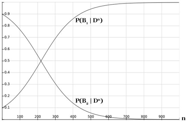
P(M | D) / P(M’ | D) = P(M) / P(M’)・P(D | M) / P(D | M’)
If M overfits the data and M’ does not, then as the size of the data set |D| goes to infinity, the likelihood factor P(D | M) / P(D | M’) goes to infinity.
Thus the posterior probability P(M | D) should go to 1 for the model that most drastically overfits the data.

This argument is wrong for a couple of reasons. For one, the argument assumes that as the size of the data set grows, the model stays the same. But this is very much not going to be true in general. The task of overfitting gets harder and harder as the number of data points go up. It’s not that there’s no longer noise in the data; it’s that the signal becomes more and more powerful.

A perfect polynomial fit on 100 data points must have, at the worst, 100 parameters. On 1000 data points: 1000 parameters. Etc. In general, as you add more data points, a model that was initially overfitting (e.g. the 100-parameter distribution) will find that it is harder and harder to ignore the signal for the noise, and the next best overfitting model will have more parameters (e.g. the 1000-parameter distribution).

But now we have a very natural solution to the problem we started with! It is true that as the number of data points increases, the evidential support for the model that overfits the data will get larger and larger. It’s also true is that the number of parameters required to overfit the data will grow as well. So if your prior in a model is a decreasing function of the number of parameters in the model, then you can in principle find a perfect balance and avoid overfitting. This perfect balance would be characterized by the following: each time you increase the number of parameters, the prior should decrease by an amount proportional to how much more you get rewarded by overfitting the data with the extra parameters.

How do we find this prior in practice? Beats me… I’d be curious to know, myself.

But what’s most interesting to me is that to solve overfitting as a Bayesian, you don’t even need the priors; the solution comes from the evidential update! It turns out that in fact, the likelihood function for updating credences in a model given data automatically incorporates in model overparameterization. Which brings us to part 2!

Part 2: Bayesian Occam’s Razor

That last sentence bears repeating. In reality, although priors can play some role by manually penalizing models with high overfitting potential, the true source of the Bayesian Occam’s razor comes from the evidential update. What we’ll find by the end of this post is that models that overfit don’t actually get a stronger evidential update than models that don’t.

You might wonder how this is possible. Isn’t it practically the definition of overfitting that it is an enhancement of the strength of an evidential update through fitting to noise in the data?

Sort of. It is super important to keep in mind the distinction between a model and a distribution. A distribution is a single probability function over your possible observable data. A model is a set of distributions, characterized by a set of parameters. When we say that some models have the potential to overfit a set of data, what we are really saying is that some models contain distributions that overfit the data.

Why is this important? Because assessing the posterior probability of the model is not the same as assessing the posterior probability of the overfitting distribution within the model! Here’s Bayes’ rule, applied to the model and to the overfitting distribution:

(1) P(M | D) = P(M)・P(D | M) / P(D)

(2) P( theta hat | D) = P()・P(D | ) / P(D)

It’s clear how to evaluate equation (2). You have some prior probability assigned to theta hat , you know how to assess the likelihood function P(D | ), and P(D) is an integral that is in principle do-able. In addition, equation (2) has the scary feature we’ve been talking about: the likelihood function P(D | ) is really really large if our parameter overfits the data, potentially large enough to swamp the priors and screw up our Bayesian calculus.

But what we’re really interested in evaluating is not equation (2), but equation (1)! This is, after all, model selection; we are in the end trying to assess the quality of different models, not individual distributions.

So how do we evaluate (1)? The key term is P(D | M); your prior over the models and the data you receive are not too important for the moment. What is P(D | M)? This question does not actually have an obvious answer… M is a model, a set of distributions, not a single distribution. If we were looking at one distribution, it would be easy to assess the likelihood of the data given that distribution.

So what does P(D | M) really mean?

It represents the average probability of the data, given the model. It’s as if you were to draw a distribution at random from your model, and see how well it fits the data. More precisely, you draw a distribution from your model, according to your prior distribution over the distributions in the model.

That was a mouthful. But the basic idea is simple; a model is an infinite set of distributions, each corresponding to a particular set of values for the parameters that define the model. You have a prior distribution over these values for the parameters, and you use this prior distribution to “randomly” select a distribution in your model. You then assess the probability of the data given that distribution, and voila, you have your likelihood function.

In other words…

P(D | M) = ∫ P(D | θ) P(θ | M) dθ

Now, an overfitting model has a massive space of parameters, and in some small region of this space contains distributions that fit the data really well. On the other hand, a simple model that generalizes well has a small space of parameters, and a region of this space contains distributions that fit the data well (though not as well as the overfitter).

So on average, you are much less likely to select the optimal distribution in the overfitting model than in the generalizable model. Why? Because the space of parameters you must search through to find it is so much larger!

True, when you do select the optimal distribution in the overfitting model, you get rewarded with a better fit to the data than you could have gotten from the nice model. But the balance, in the end, pushes you towards simpler and more general models.

This is the Bayesian Occam’s Razor! Models that are underparameterized do poorly on average, because they just can’t fit the data at all. Models that are overparametrized do poorly on average, because the subset of the parameter space that fits the data well is so tiny compared to the volume of the parameter space as a whole. And the models that strike the perfect balance are those that have enough parameters to fit the data well, but not too many as to excessively bloat the parameter space.

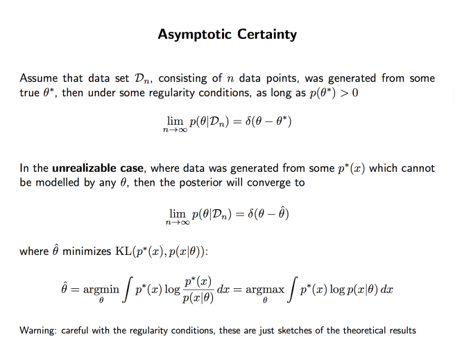
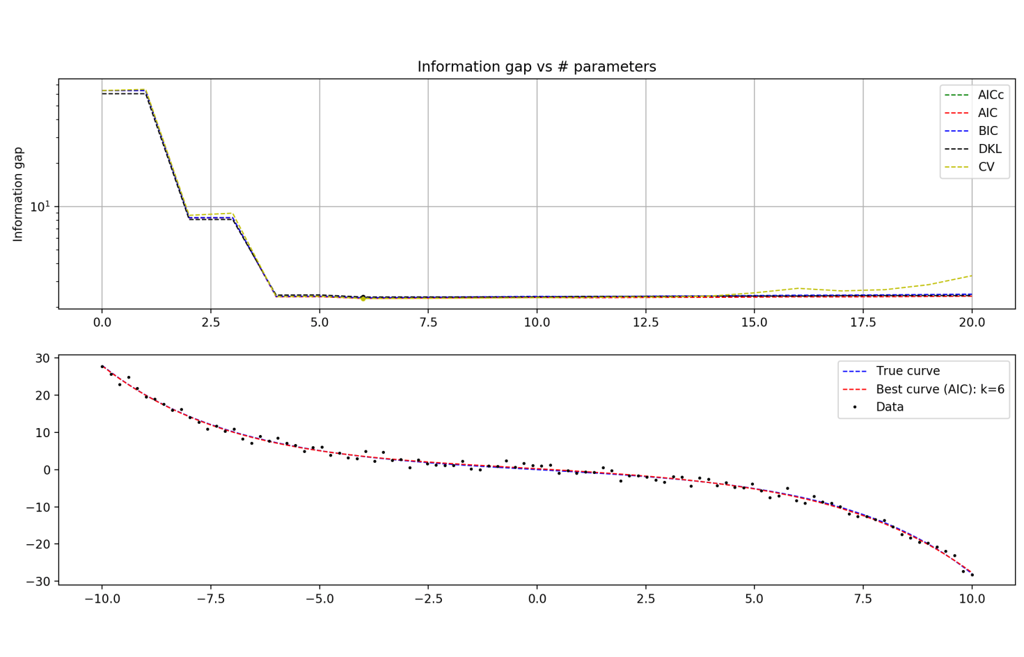
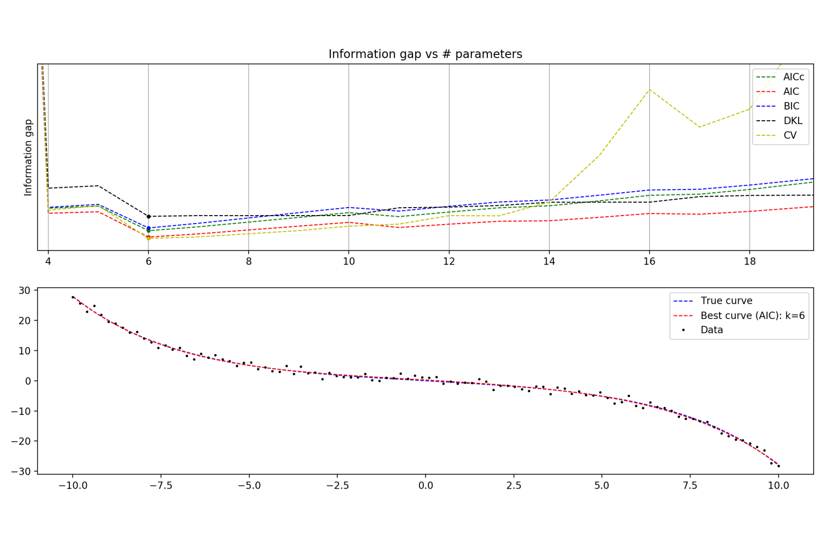
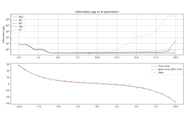
Here are some lecture slides from these great notes that have some helpful visualizations:

Screen Shot 2018-03-16 at 2.33.34 AM

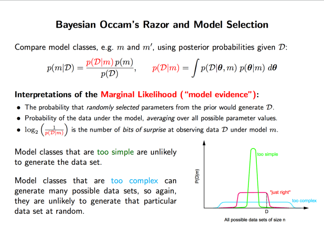
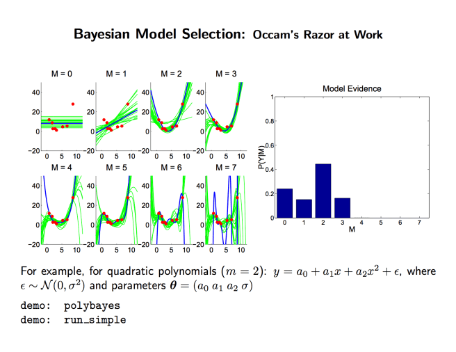
Recapping in a few sentences: Simpler models are promoted, simply because they do well on average. And evidential support for a model comes down to the performance on average, not optimal performance. The likelihood in question is not P(data | best distribution in model), it’s P(data | average distribution in model). So overfitting models actually don’t get as much evidential support from data when assessing the model quality as a whole!

Ain’t that cool??

A model selection puzzle: Why is BIC ≠ AIC?

March 14, 2018March 15, 2018 ~ squarishbracket ~ Leave a comment

Slide 19 from this lecture:

Screen Shot 2018-03-14 at 8.14.41 PM.png

This is a really important result. It says that Bayesian updating ultimately converges to the distribution in a model that minimizes D_KL, even when the truth is not in your model.

But it is also confusing to me, for the following reason.

If Bayes converges to the minimum D_KL solution, and BIC approximates Bayes, and if AIC approximately finds the minimum D_KL solution… well, then how can they give different answers?

In other words, how can all three of the following statements be true?

BIC approximates Bayes, which minimizes D_KL.
AIC approximates the minimum D_KL solution.
But BIC ≠ AIC.

Clearly we have a problem here.

It’s possible that the answer to this is just that the differences arise from the differences in approximations between AIC and BIC. But this seems like a inadequate explanation to account for such a huge difference, on the order of log(size of data set).

A friend of mine suggested that the reason is that the derivation of BIC assumes that the truth is in the set of candidate models, and this assumption is broken in the condition where Bayes’ optimizes for D_KL.

I’m not sure how strongly ‘the truth is in your set of candidate models’ is actually assumed by BIC. I know that this is the standard thing people say about BIC, but is it really that the exact truth has to be in the model, or just that the model has a low overall bias? For instance, you can derive AIC by assuming that the truth is in your set of candidate models. But you don’t need this assumption; you can also derive AIC as an approximate measure of D_KL when your set of candidate models contains models with low bias.

This question amounts to looking closely at the derivation of BIC to see what is absolutely necessary for the result. For now, I’m just pointing out the basic confusion, and will hopefully post a solution soon!

Bayes and overfitting

March 10, 2018 ~ squarishbracket ~ 2 Comments

In a couple of previous posts, I’ve said some things about Bayesianism that I now think might not be right. Specifically, I claimed a few times that Bayesians will have trouble with overfitting data. Having looked into it more and seen some complicated arguments on either side, I’m less sure about this. I’m currently just confused about it, so I’m writing up my confusion here.

The reasoning behind my initial claim was something like this:

Overfitting arises from an excessive focus on accommodation. (If your only epistemic priority is accommodating the data you receive, then you will over-accommodate the data, by fitting the noise in the data instead of just the underlying trend.)
We can deal with overfitting by optimizing for other epistemic virtues like simplicity, predictive accuracy, or some measure of distance to truth. (For example, minimum description length and maximum entropy optimize for simplicity, and cross validation optimizes for predictive accuracy).
Bayesianism is an epistemological procedure that has two steps, setting of priors and updating those priors.
Updating of priors is done via Bayes’ rule, which rewards theories according to how well they accommodate their data (creating the potential for overfitting).
Bayesian priors can be set in ways that optimize for other epistemic virtues, like simplicity or humility.
In the limit of infinite evidence, differences in priors between empirically distinguishable theories are washed away.
Thus, in the limit, Bayesianism becomes a primarily accommodating procedure, as the strength of the evidential update swamps your initial differences in priors.

In other words, the model that is best supported by the data will be the one that fits it perfectly (i.e. overfitting). We get out of this by giving overfitting models low priors… but we should expect that even this won’t be sufficient if we get strong enough evidence.

Is this wrong? And why?

More model selection visualizations

March 8, 2018June 4, 2018 ~ squarishbracket ~ Leave a comment

I added cross validation to my model selection program, and ooh boy do I now understand why people want to find more efficient alternatives.

Reliable CV calculations end up making the program run orders of magnitude slower, as they require re-fitting the curve for every partition of your data and this is the most resource-intensive part of the process. While it’s beautiful in theory, this is a major set-back in practice.

For a bunch of different true distributions I tried, I found that CV pretty much always lines up with all of the other methods, just with a more “jagged” curve and a steeper complexity penalty. This similarity looks like a score for the other methods, assuming that CV does a good job of measuring predictive power. (And for those interested in the technical details, the cross validation procedure implemented here is leave-one-out CV)

I also added an explicit calculation of D_KL, which should help to give some idea of a benchmark against which we can measure all of these methods. Anyway, I have some more images!

True curve = e^-x/3 – e^x/3

N = 100 data points

N = 100 data points, zoomed in a bit

For smaller data sets, you can see that AICc tracks D_KL much more closely than any other technique (which is of course the entire purpose of AICc).

N = 25

N = 25, zoomed

N = 25, super zoom

Interestingly, you start to see BIC really suffering relative to the other methods, beginning to overfit the data. This is counterintuitive; BIC is supposed to be the method that penalizes complexity excessively and underfits the data. Relevant is that in this program, I use the form of BIC that doesn’t approximate for large N.

BIC_{small N} = k log(N/2π) – 2L
BIC_ordinary = k log(N) – 2L

When I use the approximation instead, the problem disappears. Of course, this is not too great a solution; why should the large N approximation be necessary for fixing BIC specifically when N is small?

(Edit: after many more runs, it’s looking more like it may have just been a random accident that BIC overfit in the first few runs)

Just for the heck of it, I also decided to torture my polynomials a little bit by making them try to fit the function 1/x. I got dismal results no matter how I tried to tweak the hyper-parameters, which is, well, pretty much what I expected (1/x has no Taylor expansion around 0, for one thing).

More surprisingly, I tried fitting a simple Gaussian curve and again got fairly bad results. The methods disagreed with one another a lot of the time (although weirdly, AICc and BIC seemed to generally be in agreement), and gave curves that were overfitting the data a bit. The part that seems hardest for a polynomial to nail down is the flattened ends of the Gaussian curve.

True curve = 40 exp(-x²/2), N = 100 data points

And zoomed in…

If the jaggedness of the cross validation score is not purely an artifact of random fluctuations in the data, I don’t really get it. Why should, for example, a 27-parameter model roughly equal a 25-parameter model in predictive power, but a 26-parameter model be significantly worse than both?

The Monty Hall non-paradox

March 6, 2018March 15, 2018 ~ squarishbracket ~ 1 Comment

I recently showed the famous Monty Hall problem to a friend. This friend solved the problem right away, and we realized quickly that the standard presentation of the problem is highly misleading.

Here’s the setup as it was originally described in the magazine column that made it famous:

Suppose you’re on a game show, and you’re given the choice of three doors: Behind one door is a car; behind the others, goats. You pick a door, say No. 1, and the host, who knows what’s behind the doors, opens another door, say No. 3, which has a goat. He then says to you, “Do you want to pick door No. 2?” Is it to your advantage to switch your choice?

I encourage you to think through this problem for yourself and come to an answer. Will provide some blank space so that you don’t accidentally read ahead.

…

Now, the writer of the column was Marilyn vos Savant, famous for having an impossible IQ of 228 according to an interpretation of a test that violated “almost every rule imaginable concerning the meaning of IQs” (psychologist Alan Kaufman). In her response to the problem, she declared that switching gives you a 2/3 chance of winning the car, as opposed to a 1/3 chance for staying. She argued by analogy:

Yes; you should switch. The first door has a 1/3 chance of winning, but the second door has a 2/3 chance. Here’s a good way to visualize what happened. Suppose there are a million doors, and you pick door #1. Then the host, who knows what’s behind the doors and will always avoid the one with the prize, opens them all except door #777,777. You’d switch to that door pretty fast, wouldn’t you?

Notice that this answer contains a crucial detail that is not contained in the statement of the problem! Namely, the answer adds the stipulation that the host “knows what’s behind the doors and will always avoid the one with the prize.”

The original statement of the problem in no way implies this general statement about the host’s behavior. All you are justified to assume in an initial reading of the problem are the observational facts that (1) the host happened to open door No. 3, and (2) this door happened to contain a goat.

When nearly a thousand PhDs wrote in to the magazine explaining that her answer was wrong, she gave further arguments that failed to reference the crucial point; that her answer was only true given additional unstated assumptions.

My original answer is correct. But first, let me explain why your answer is wrong. The winning odds of 1/3 on the first choice can’t go up to 1/2 just because the host opens a losing door. To illustrate this, let’s say we play a shell game. You look away, and I put a pea under one of three shells. Then I ask you to put your finger on a shell. The odds that your choice contains a pea are 1/3, agreed? Then I simply lift up an empty shell from the remaining other two. As I can (and will) do this regardless of what you’ve chosen, we’ve learned nothing to allow us to revise the odds on the shell under your finger.

Notice that this argument is literally just a restatement of the original problem. If one didn’t buy the conclusion initially, restating it in terms of peas and shells is unlikely to do the trick!

This problem was made even more famous by this scene in the movie “21”, in which the protagonist demonstrates his brilliance by coming to the same conclusion as vos Savant. While the problem is stated slightly better in this scene, enough ambiguity still exists that the proper response should be that the problem is underspecified, or perhaps a set of different answers for different sets of auxiliary assumptions.

The wiki page on this ‘paradox’ describes it as a veridical paradox, “because the correct choice (that one should switch doors) is so counterintuitive it can seem absurd, but is nevertheless demonstrably true.”

Later on the page, we see the following:

In her book The Power of Logical Thinking, vos Savant (1996, p. 15) quotes cognitive psychologist Massimo Piattelli-Palmarini as saying that “no other statistical puzzle comes so close to fooling all the people all the time,” and “even Nobel physicists systematically give the wrong answer, and that they insist on it, and they are ready to berate in print those who propose the right answer.”

There’s something to be said about adequacy reasoning here; when thousands of PhDs and some of the most brilliant mathematicians in the world are making the same point, perhaps we are too quick to write it off as “Wow, look at the strength of this cognitive bias! Thank goodness I’m bright enough to see past it.”

In fact, the source of all of the confusion is fairly easy to understand, and I can demonstrate it in a few lines.

Solution to the problem as presented

Initially, all three doors are equally likely to contain the car.
So Pr(1) = Pr(2) = Pr(3) = ⅓

We are interested in how these probabilities update upon the observation that 3 does not contain the car.
Pr(1 | ~3) = Pr(1)・Pr(~3 | 1) / Pr(~3)
= (⅓ ・1) / ⅔ = ½

By the same argument,
Pr(2 | ~3) = ½

Voila. There’s the simple solution to the problem as it is presented, with no additional presumptions about the host’s behavior. Accepting this argument requires only accepting three premises:

(1) Initially all doors are equally likely to be hiding the car.

(2) Bayes’ rule.

(3) There is only one car.

(3) implies that Pr(the car is not behind a door | the car is behind a different door) = 100%, which we use when we replace Pr(~3 | 1) with 1.

The answer we get is perfectly obvious; in the end all you know is that the car is either in door 1 or door 2, and that you picked door 1 initially. Since which door you initially picked has nothing to do with which door the car was behind, and the host’s decision gives you no information favoring door 1 over door 2, the probabilities should be evenly split between the two.

It is also the answer that all the PhDs gave.

Now, why does taking into account the host’s decision process change things? Simply because the host’s decision is now contingent on your decision, as well as the actual location of the car. Given that you initially opened door 1, the host is guaranteed to not open door 1 for you, and is also guaranteed to not open up a door hiding the car.

Solution with specified host behavior

Initially, all three doors are equally likely to contain the car.
So Pr(1) = Pr(2) = Pr(3) = ⅓

We update these probabilities upon the observation that 3 does not contain the car, using the likelihood formulation of Bayes’ rule.

Pr(1 | open 3) / Pr(2 | open 3)
= Pr(1) / Pr(2)・Pr(open 3 | 1) / Pr(open 3 | 2)
= ⅓ / ⅓・½ / 1 = ½

So Pr(1 | open 3) = ⅓ and Pr(2 | open 3) = ⅔

Pr(open 3 | 2) = 1, because the host has no choice of which door to open if you have selected door 1 and the car is behind door 2.

Pr(open 3 | 1) = ½, because the host has a choice of either opening 2 or 3.

In fact, it’s worth pointing out that this requires another behavioral assumption about the host that is nowhere stated in the original post, or Savant’s solution. This is that if there is a choice about which of two doors to open, the host will pick randomly.

This assumption is again not obviously correct from the outset; perhaps the host chooses the larger of the two door numbers in such cases, or the one closer to themselves, or the one or the smaller number with 25% probability. There are an infinity of possible strategies the host could be using, and this particular strategy must be explicitly stipulated to get the answer that Wiki proclaims to be correct.

It’s also worth pointing out that once these additional assumptions are made explicit, the ⅓ answer is fairly obvious and not much of a paradox. If you know that the host is guaranteed to choose a door with a goat behind it, and not one with a car, then of course their decision about which door to open gives you information. It gives you information because it would have been less likely in the world where the car was under door 1 than in the world where the car was under door 2.

In terms of causal diagrams, the second formulation of the Monty Hall problem makes your initial choice of door and the location of the car dependent upon one another. There is a path of causal dependency that goes forwards from your decision to the host’s decision, which is conditioned upon, and then backward from the host’s decision to which door the car is behind.

Any unintuitiveness in this version of the Monty Hall problem is ultimately due to the unintuitiveness of the effects of conditioning on a common effect of two variables.

Monty Hall Causal

In summary, there is no paradox behind the Monty Hall problem, because there is no single Monty Hall problem. There are two different problems, each containing different assumptions, and each with different answers. The answers to each problem are fairly clear after a little thought, and the only appearance of a paradox comes from apparent disagreements between individuals that are actually just talking about different problems. There is no great surprise when ambiguous wording turns out multiple plausible solutions, it’s just surprising that so many people see something deeper than mere ambiguity here.

A note of ambiguity regarding model selection

March 3, 2018April 19, 2018 ~ squarishbracket ~ Leave a comment

A model is a family of probability distributions over a set of observable variables X, parameterized by some set of parameters a₁, a₂, …, a_k.

M = { p(X | a₁, a₂, …, a_k) | ∀ a₁, a₂, …, a_k }

Models arise naturally when we are unsure about some details of a distribution, but know its general form. For example, maybe we know that the positions of particles in a gas cloud are normally distributed, but don’t know the degree of spread of this cloud or the location of its center. Then we would want to represent the positions of our particles by a Gaussian distribution over all possible positions, parameterized by the mean and variance of the distribution.

Given this model, we can now make observations of particle positions in order to gain information about the spread and center of the gas cloud. In other words, we have split our epistemological task into two questions:

What model is best? (Model selection)
What values of the parameters are best? (Parameter selection)

Parameter selection is generally accomplished by ordinary accommodation procedures. Broadly, these fall into two categories:

Likelihood maximization (which parameters make the data most likely?)
Posterior maximization (which parameters are made most likely by the data?)

Model selection is where we correct for overfitting and prioritize simplicity. Two common optimization goals are:

Minimize information divergence (which model is closest to the truth in information theoretic terms?)
Maximize predictive accuracy (which model does the best job at predicting the next data point?)

So to summarize, we decide what to believe by (1) selecting a set of models, (2) optimizing each model to fit our data, and (3) comparing our optimized models using model selection criteria.

Now, while (3) and (2) are perfectly clear to me, (1) seems much less so. How do we decide what set of models we are working with? While this might be easily practically solved by just using a standard set of models, it seems theoretically troubling. One problem is that the space of possible models is incredibly large, and can be divided up in many different ways.

Another problem is that two people that are looking at all the same hypotheses might have apparent disagreements about what models they are using. Let’s look at an example of this. Person A and Person B both are looking at the same hypothesis set: the set of all lines through the origin with a Gaussian measurement error. But they describe their epistemic framework as follows:

Person A: I have a single model, defined by a single parameter: M = { y = ax + U | a ∈ ℝ, U a Gaussian error term }.

Person B: I have an uncountable infinity of models, each defined by zero parameters. Labeling each model with index a ∈ ℝ, I can describe the a^th model: M_a = { y = ax + U | U a Gaussian error term }.

The difference between these two is clearly purely semantic; both are looking at the same set of hypotheses, but one is considering them to be contained in a single overarching model, and the other is looking at them each individually.

This becomes a problem when we consider the fact that model selection techniques are sensitive to the number of parameters in the model. More parameters = a larger penalty for overfitting. So while Person A will be penalized for having one tweakable parameter, Person B will be free from penalty.

The response that we want to give here is that Person B is really working with a single model in all but name. What we really care about is the ability of an agent to search among a large space of models, with the excessive flexibility that allows them to not only identify trends in data but also to track the noise in the data. And both Person A and Person B have equal flexibility in this regard, so should be penalized accordingly.

We could try to implement this formally by attempting to reduce large sets of models to smaller sets as much as possible. The problem with this is that any set of models can in principle be reduced to a single larger model with additional adjustable parameters.

In general, the problem of how to clearly distinguish between parameters and models seems like a fairly serious issue for any epistemology that fundamentally relies on this distinction.

Gibbs’ inequality

March 2, 2018March 2, 2018 ~ squarishbracket ~ 1 Comment

As a quick reminder from previous posts, we can define the surprise in an occurrence of an event E with probability P(E) as:

Sur(P(E)) = log(1/P) = – log(P).

I’ve discussed why this definition makes sense here. Now, with this definition, we can talk about expected surprise; in general, the surprise that somebody with distribution Q would expect somebody with distribution P to have is:

E_Q[Sur(P)] = ∫ – Q log(P) dE

This integral is taken over all possible events. A special case of it is entropy, which is somebody’s own expected surprise. This corresponds to the intuitive notion of uncertainty:

Entropy = E_P[Sur(P)] = ∫ – P log(P) dE

The actual average surprise for somebody with distribution P is:

Actual average surprise = ∫ – P_true log(P) dE

Here we are using the idea of a true probability distribution, which corresponds to the distribution over possible events that best describes the frequencies of each event. And finally, the “gap” in average surprise between P and Q is:

∫ P_true log(P/Q) dE

Gibbs’ inequality says the following:

For any two different probability distributions P and Q:
E_P[Sur(P)] < E_P[Sur(Q)]

This means that out of all possible ways of distributing your credences, you should always expect that your own distribution is the least surprising.

In other words, you should always expect to be less surprised than everybody else.

This is really unintuitive, and I’m not sure how to make sense of it. Say that you think that a coin will either land heads or tails, with probability 50% for each. In addition, you are with somebody (who we’ll call A) that you know has perfect information about how the coin will land.

Does it make sense to say that you expect them to be more surprised about the result of the coin flip than you will be? This seems hardly intuitive. One potential way out of this is that the statement “A knows exactly how the coin will land” has not actually been included in your probability distribution, so it isn’t fair to stipulate that you know this. One way to try to add in this information is to model their knowledge by something like “There’s a 50% chance that A’s distribution is 100% H, and a 50% chance that it is 100% T.”

The problem is that when you average over these distributions, you get a new distribution that is identical to your own. This is clearly not capturing the state of knowledge in question.

Another possibility is that we should not be thinking about the expected surprise of people, but solely of distributions. In other words, Gibb’s inequality tells us that you will expect a higher average surprise for any distribution that you are handed, than for your own distribution. This can only be translated into statements about people‘s average surprise when their knowledge can be directly translated into a distribution.

Bayes and beyond

February 23, 2018March 15, 2018 ~ squarishbracket ~ Leave a comment

You have lots of beliefs about the world. Each belief can be written as a propositional statement that is either true or false. But while each statement is either true or false, your beliefs are more complicated; they come in shades of gray, not blacks and whites. Instead of beliefs being on-or-off, we have degrees of beliefs – some beliefs are much stronger than others, some have roughly the same degree of belief, and so on. Your smallest degrees of belief are for true impossibilities – things that you can be absolutely certain are false. Your largest degrees of beliefs are for absolute certainties, the other side of the coin.

Now, answer for yourself the following series of questions:

Can you quantify a degree of belief?

By quantify, I mean put a precise, numerical value on it. That is, can you in principle take any belief of yours, and map it to a real number that represents how strongly you believe it? The in principle is doing a lot of work here; maybe you don’t think that you can in practice do this, but does it make conceptual sense to you to think about degrees of belief as quantities?

If so, then we can arbitrarily scale your degrees of belief by translating them into what I’ll call for the moment credences. All of your credences are on a scale from 0 to 1, where 0 is total disbelief and 1 is totally certain belief. We can accomplish this rescaling by just shifting all your degrees of belief up by your lowest degree of belief (that which you assign to logical impossibilities), and then dividing each degree of belief by the difference between your most distant degrees of belief.

Now,

If beliefs B and B’ are mutually exclusive (i.e. it is impossible for them both to be true), then do you agree that your credence in one of the two of them being true should be the sum of your credences in each individually?

Said more formally, do you agree that if Cr(B & B’) = 0, then Cr(B or B’) = Cr(B) + Cr(B’)? (The equal sign here should be a normative equals sign. We are not asking if you think this is descriptively true of your degrees of beliefs, but if you think that this should be true of your degrees of beliefs. This is the normativity of rationality, by the way, not ethics.)

If so, then your credence function Cr is really a probability function (Cr(B) = P(B)). With just these two questions and the accompanying comments, we’ve pinned down the Kolmogorov axioms for a simple probability space. But we’re not done!

Next,

Do you agree that your credence in two statements B and B’ both being true should be your credence in B’ given that B is true, multiplied by your credence in B?

Formally: Do you agree that P(B & B’) = P (B’ | B) ∙ P(B)? If you haven’t seen this before, this might not seem immediately intuitively obvious. It can be made so quite easily. To find out how strongly you believe both B and B’, you can firstly imagine a world in which B is true and judge your credence in B’ in this scenario, and then secondly judge your actual credence in B being the real world. The conditional probability is important here in order to make sure you are not ignoring possible ways that B and B’ could depend upon each other. If you want to know the chance that both of somebody’s eyes are brown, you need to know (1) how likely it is that their left eye is brown, and (2) how likely it is that their right eye is brown, given that their left eye is brown. Clearly, if we used an unconditional probability for (2), we would end up ignoring the dependency between the colors of the right and left eye.

Still on board? Good! Number 3 is crucially important. You see, the world is constantly offering you up information, and your beliefs are (and should be) constantly shifting in response. We now have an easy way to incorporate these dynamics.

Say that you have some initial credence in a belief B about whether you will experience E in the next few moments. Now you see that after a few moments pass, you did experience E. That is, you discover that B is true. We can now set P(B) equal to 1, and adjust everything else accordingly:

For all beliefs B’, P_new(B’) = P(B’ | B)

In other words, your new credences are just your old credences given the evidence you received. What if you weren’t totally sure that B is true? Maybe you want P(B) = .99 instead. Easy:

For all beliefs B’: P_new(B’) = .99 ∙ P(B’ | B) + .01 ∙ P(B’ | ~B)

In other words, your new credence in B’ is just your credence that B is true, multiplied by the conditional credence of B’ given that B is true, added to your credence that B is false times the conditional credence of B’ given that B is false.

We now have a fully specified general system of updating beliefs; that is, we have a mandated set of degrees of beliefs at any moment after some starting point. But what of this starting point? Is there a rationally mandated prior credence to have, before you’ve received any evidence at all? I.e., do we have some a priori favored set of prior degrees of belief?

Intuitively, yes. Some starting points are obviously less rational than others. If somebody starts off being totally certain in the truth of one side of an a posteriori contingent debate that cannot be settled as a matter of logical truth, before receiving any evidence for this side, then they are being irrational. So how best to capture this notion of normative rational priors? This is the question of objective Bayesianism, and there are several candidates for answers.

One candidate relies on the notions of surprise and information. Since we start with no information at all, we should start with priors that represent this state of knowledge. That is, we want priors that represent maximum uncertainty. Formalizing this notion gives us the principle of maximum entropy, which says that the proper starting point for beliefs is that which maximizes the entropy function ∑ -P logP.

There are problems with this principle, however, and many complicated debates comparing it to other intuitively plausible principles. The question of objective Bayesianism is far from straightforward.

Putting aside the question of priors, we have a formalized system of rules that mandates the precise way that we should update our beliefs from moment to moment. Some of the mandates seem unintuitive. For instance, it tells us that if we get a positive result on a 99% accurate test for a disease with a 1% prevalence rate, then we have a 50% chance of having the disease, not 99%. There are many known cases where our intuitive judgments of likelihood differ from the judgments that probability theory tells us are rational.

How do we respond to these cases? We only really have a few options. One, we could discard our formalization in favor of the intuitions. Two, we could discard our intuitions in favor of the formalization. Or three, we could accept both, and be fine with some inconsistency in our lives. Presuming that inconsistency is irrational, we have to make a judgment call between our intuitions and our formalization. Which do we discard?

Remember, our formalization is really just the necessary result of the set of intuitive principles we started with. So at the core of it, we’re really just comparing intuitions of differing strengths. If your intuitive agreement with the starting principles was stronger than your intuitive disagreement with the results of the formalization, then presumably you should stick with the formalization.

Another path to adjudicating these cases is to consider pragmatic arguments for our formalization, like Dutch Book arguments that indicate that our way of assigning degrees of beliefs is the only one that is not exploitable by a bookie to ensure losses. You can also be reassured by looking at consistency and convergence theorems, that show the Bayesian’s beliefs converging to the truth in a wide variety of cases.

If you’re still with me, you are now a Bayesian. What does this mean? It means that you think that it is rational to treat your beliefs like probabilities, and that you should update your beliefs by conditioning upon the evidence you receive.

***

So what’s next? Are we done? Have all epistemological issues been solved? Unfortunately not. I think of Bayesianism as a first step into the realm of formal epistemology – a very good first step, but nonetheless still a first. Here’s a simple example of where Bayesianism will lead us into apparent irrationality.

Imagine we have two different beliefs about the world: B₁ and B₂. B₂ is a respectable scientific theory: one that puts its neck out with precise predictions about the results of experiments, and tries to identify a general pattern in the underlying phenomenon. B₁ is a “cheating” theory: it doesn’t have any clue what’s going to happen before an experiment, but after an experiment it peeks at the results and pretends that it had predicted it all along. We might think of B₁ as the theory that perfectly fits all of the data, but only through over-fitting on the data. As such, B₁ is unable to make any good predictions about future data.

What does Bayesianism say about these two theories? Well, consider any single data point. Let’s suppose that B₂ does a good job predicting this data point, say, P(D | B₂) = 99%. And since B₁ perfectly fits the data, P(D | B₁) = 1. If our priors in B₁ and B₂ are written as P₁ and P₂, respectively, then our credences update as follows:

P_new(B₁) = P(B₁ | D) = P₁ / (P₁ + .99 P₂)
P_new(B₂) = P(B₂ | D) = .99 P₂ / (P₁ + .99 P₂)

For N similar data points, we get:

P_new(B₁) = P(B₁ | Dⁿ) = P₁ / (P₁ + .99ⁿ P₂)
P_new(B₂) = P(B₂ | Dⁿ) = .99ⁿ P₂ / (P₁ + .99ⁿ P₂)

What happens to these two credences as n gets larger and larger?

Bayes and beyond

As we can see, our credence in B₁ approaches 100% exponentially quickly, and our credence in B₂ drops to 0% exponentially quickly. Even if we start with an enormously low prior in B₁, our credence will eventually be swamped as we gather more and more data.

It looks like in this example, the Bayesian is successfully hoodwinked by the cheating theory, B₁. But this is not quite the end of the story for Bayes. The only single theory that perfectly predicts all of the data you receive in the infinite evidence limit is basically just the theory that “Everything that’s going to happen is what’s going to happen.” And, well, this is surely true. It’s just not very useful.

If instead we look at B₁ as a sequence of theories, one for each new data point, then we have a way out by claiming that our priors drop as we go further in the sequence. This is an appeal to simplicity – a theory that exactly specifies 1000 different data points is more complex than a theory that exactly specifies 100 different data points. It also suggests a precise way to formalize simplicity, by encoding it into our priors.

While the problem of over-fitting is not an open-and-shut case against Bayesianism, it should still give us pause. The core of the issue is that there are more intuitive epistemic virtues than those that the Bayesian optimizes for. Bayesianism mandates a degree of belief as a function of two ingredients: the prior and the evidential update. The second of these, Bayesian updating, solely optimizes for accommodation of data. And setting of priors is typically done to optimize for some notion of simplicity. Since empirically distinguishable theories have their priors washed out in the limit of infinite evidence, Bayesianism becomes a primarily accommodating epistemology.

This is what creates the potential for problems of overfitting to arise. The Bayesian is only optimizing for accommodation and simplicity, but what we want is a framework that also optimizes for prediction. I’ll give two examples of ways to do this: cross validation and posterior predictive checking.

I’ve talked about cross validation previously. The basic idea is that you split a set of data into a training set and a testing set, optimize your model for best fit with the training set, and then see how it performs on the testing set. In doing so, you are in essence estimating how well your model will do on predictions of future data points.

This procedure is pretty commonsensical. Want to know how well your model does at predicting data? Well, just look at the predictions it makes and evaluate how accurate they were. It is also completely outside of standard Bayesianism, and solves the issues of overfitting. And since the first half of cross validation is training your model to fit the training set, it is optimizing for both accommodation and prediction.

Posterior predictive checks are also pretty commonsensical; you ask your model to make predictions for future data, and then see how these predictions line up with the data you receive.

More formally, if you have some set of observable variables X and some other set of parameters A that are not directly observable, but that influence the observables, you can express your prior knowledge (before receiving data) as a prior over A, P(A), and a likelihood function P(X | A). Upon receiving some data D about the values of X, you can update your prior over A as follows:

P(A) becomes P(A | D)
where P(A | D) = P(D | A) P(A) / P(D)

To make a prediction about how likely you think it is that the next data point will be X, given the data D, you must use the posterior predictive distribution:

P(X | D) = ∫ P(X | A) ∙ P(A | D) dA

This gives you a precise probability that you can use to evaluate the predictive accuracy of your model.

There’s another goal that we can aim towards, besides accommodation, simplicity, or prediction. This is distance from truth. You might think that this is fairly obvious as a goal, and that all the other methods are really only attempts to measure this. But in information theory, there is a precise way in which you can specify the information gap between any given theory and reality. This metric is called the Kullback-Leibler divergence (D_KL), and I’ll refer to it as just information divergence.

D_KL = ∫ P_true log(P_true / P) dx

This term, if parsed correctly, represents precisely how much information you gain if you go from your starting distribution P to the true distribution P_true.

For example, if you have a fair coin, then the true distribution is given by (P_true(H) = .5, P_true(T) = .5). You can calculate how far any other theory (P(H) = p, P(T) = 1 – p) is from the truth using D_KL.

D_KL = .5 ∙ [ log(1 / 2p) + log(1 / 2(1-p)) ]

I’ve graphed D_KL as a function of p here:

Information divergence.png

As you can see, the information divergence is 0 for the correct theory that the coin is fair (p = 0.5), and goes to infinity as you get further away from this.

This is all well and good, but how is this practically applicable? It’s easy to minimize the distance from the true distribution if you already know the true distribution, but the problem is exactly that we don’t know the truth and are trying to figure it out.

Since we don’t have direct access to P_true, we must resort to approximations of D_KL. The most famous approximation is called the Akaike information criterion (AIC). I won’t derive the approximation here, but will present the form of this quantity.

AIC = k – log(P(data | M))
where M = the model being evaluated
and k = number of parameters in M

The model that minimizes this quantity probably also minimizes the information distance from truth. Thus, “lower AIC value” serves as a good approximation to “closer to the truth”. Notice that AIC explicitly takes into account simplicity; the quantity k tells you about how complex a model is. This is pretty interesting in it’s own right; it’s not obvious why a method that is solely focused on optimizing for truth will end up explicitly including a term that optimizes for simplicity.

Here’s a summary table describing the methods I’ve talked about here (as well as some others that I haven’t talked about), and what they’re optimizing for.

Goal	Method(s)
Which theory makes the data most likely?	Maximum likelihood estimation (MLE) p-testing
Which theory is most likely, given the data?	Bayes Bayesian information criterion (BIC)
Maximum uncertainty	Entropy Relative entropy
Simplicity	Minimum description length Solomonoff induction
Predictive accuracy	Cross validation Posterior predictive checks
Distance from truth	Information divergence (D_KL) Akaike information criterion (AIC)

A simple explanation of Bell’s inequality

February 14, 2018December 27, 2018 ~ squarishbracket ~ 2 Comments

Everybody knows that quantum mechanics is weird. But there are plenty of weird things in the world. We’ve pretty much come to expect that as soon as we look out beyond our little corner of the universe, we’ll start seeing intuition-defying things everywhere. So why does quantum mechanics get the reputation of being especially weird?

Bell’s theorem is a good demonstration of how the weirdness of quantum mechanics is in a realm of its own. It’s a set of proposed (and later actually verified) experimental results that seem to defy all attempts at classical interpretation.

The Experimental Results

Here is the experimental setup:

Bell

In the center of the diagram, we have a black box that spits out two particles every few minutes. These two particles fly in different directions to two detectors. Each detector has three available settings (marked by 1, 2, and 3) and two bulbs, one red and the other green.

Shortly after a particle enters the detector, one of the two bulbs flashes. Our experiment is simply this: we record which bulb flashes on both the left and right detector, and we take note of the settings on both detectors at the time. We then try randomly varying the detector settings, and collect data for many such trials.

Quick comprehension test: Suppose that what bulb flashes is purely a function of some property of the particles entering the detector, and the settings don’t do anything. Then we should expect that changes in the settings will not have any impact on the frequency of flashing for each bulb. It turns out that we don’t see this in the experimental results.

One more: Suppose that the properties of the particles have nothing to do with which bulb flashes, and all that matters is the detector settings. What do we expect our results to be in this case?

Well, then we should expect that changing the detector settings will change which bulb flashes, but that the variance in the bulb flashes should be able to be fully accounted for by the detector settings. It turns out that this also doesn’t happen.

Okay, so what do we see in the experimental results?

The results are as follows:

(1) When the two detectors have the same settings:
The same color of bulb always flashes on the left and right.

(2) When the two detectors have different settings:
The same color bulb flashes on the left and right 25% of the time.
The same color bulb flashes on the left and right 75% of the time.

In some sense, the paradox is already complete. It turns out that some very minimal assumptions about the nature of reality tell us that these results are impossible. There is a hidden inconsistency within these results, and the only remaining task is to draw it out and make it obvious.

Assumptions

We’ll start our analysis by detailing our basic assumptions about the nature of the process.

Assumption 1: Lawfulness
The probability of an event is a function of all other events in the universe.

This assumption is incredibly weak. It just says that if you know everything about the universe, then you are able to place a probability distribution over future events. This isn’t even as strong as determinism, as it’s only saying that the future is a probabilistic function of the past. Determinism would be the claim that all such probabilities are 1 or 0, that is, the facts about the past fix the facts about the future.

From Assumption 1 we conclude the following:

There exists a function P(R | everything else) that accurately reports the frequency of the red bulb flashing, given the rest of facts about the universe.

It’s hard to imagine what it would mean for this to be wrong. Even in a perfectly non-deterministic universe where the future is completely probabilistically independent of the past, we could still express what’s going to happen next probabilistically, just with all of the probabilities of events being independent. This is why even naming this assumption lawfulness is too strong – the “lawfulness” could be probabilistic, chaotic, and incredibly minimal.

The next assumption constrains this function a little more.

Assumption 2: Locality
The probability of an event only depends on events local to it.

This assumption is justified by virtually the entire history of physics. Over and over we find that particles influence each others’ behaviors through causal intermediaries. Einstein’s Special Theory of Relativity provides a precise limitation on causal influences; the absolute fastest that causal influences can propagate is the speed of light. The light cone of an event is defined as all the past events that could have causally influenced it, given the speed of light limit, and all future events that can be causally influenced by this event.

Combining Assumption 1 and Assumption 2, we get:

P(R | everything else) = P(R | local events)

So what are these local events? Given our experimental design, we have two possibilities; the particle entering the detector, and the detector settings. Our experimental design explicitly rules out the effects of other causal influences, by holding them fixed. The only thing that we, the experimenters, vary are the detector settings, and the variation in the particle types being produced by the central black box. All else is stipulated to be held constant.

Thus we get our third, and final assumption.

Assumption 3: Good experimental design
The only local events relevant to the bulb flashing are the particle that enters the detector and the detector setting.

Combining these three assumptions, we get the following:

P(R | everything else) = P(R | particle & detector setting)

We can think of this function a little differently, by asking about a particular particle with a fixed set of properties.

P_particle(R | detector setting)

We haven’t changed anything but the notation – this is the same function as what we originally had, just carrying a different meaning. Now it tells us how likely a given particle is to cause the red bulb to flash, given a certain detector setting. This allows us to categorize all different types of particles by looking at all different settings.

Particle type is defined by
( P_particle(R | Setting 1), P_particle(R | Setting 2), P_particle(R | Setting 3) )

This fully defines our particle type for the purposes of our experiment. The set of particle types is the set of three-tuples of probabilities.

So to summarize, here are the only three assumptions we need to generate the paradox.

Lawfulness: Events happen with probabilities that are determined by facts about the universe.
Locality: Causal influences propagate locally.
Good experimental design: Only the particle type and detector setting influence the experiment result.

Now, we generate a contradiction between these assumptions and the experimental results!

Contradiction

Recall our experimental results:

(1) When the two detectors have the same settings:
The same color of bulb always flashes on the left and right.

(2) When the two detectors have different settings:
The same color bulb flashes on the left and right 25% of the time.
The same color bulb flashes on the left and right 75% of the time.

We are guaranteed by Assumptions 1 to 3 that there exists a function P_particle(R | detector setting) that describes the frequencies we observe for a detector. We have two particles and two detectors, so we are really dealing with two functions for each experimental trial.

Left particle: P_left(R | left setting)
Right particle: P_right(R | right setting)

From Result (1), we see that when left setting = right setting, the same color always flashes on both sides. This means two things: first, that the black box always produces two particles of the same type, and second, that the behavior observed in the experiment is deterministic.

Why must they be the same type? Well, if they were different, then we would expect different frequencies on the left and the right. Why determinism? If the results were at all probabilistic, then even if the probability functions for the left and right particles were the same, we’d expect to still see them sometimes give different results. Since they don’t, the results must be fully determined.

This means that we can fully express particle types by a function that takes in a setting (1, 2, or 3), and returns a value (0 or 1) corresponding to whether or not the red bulb will flash. How many different types of particles are there? Eight!

Abbreviation: P_n = P(R | setting n)
P₁ = 1, P₂ = 1, P₃ = 1 : (RRR)
P₁ = 1, P₂ = 1, P₃ = 0 : (RRG)
P₁ = 1, P₂ = 0, P₃ = 1 : (RGR)
P₁ = 1, P₂ = 0, P₃ = 0 : (RGG)
P₁ = 0, P₂ = 1, P₃ = 1 : (GRR)
P₁ = 0, P₂ = 1, P₃ = 0 : (GRG)
P₁ = 0, P₂ = 0, P₃ = 1 : (GGR)
P₁ = 0, P₂ = 0, P₃ = 0 : (GGG)

The three-letter strings (RRR) are short representations of which bulb will flash for each detector setting.

Now we are ready to bring in experimental result (2). In 25% of the cases in which the settings are different, the same bulbs flash on either side. Is this possible given our results? No! Check out the following table that describes what happens with RRR-type particles and RRG-type particles when the detectors have different settings different detector settings.

(Setting 1, Setting 2)	RRR-type	RRG-type
1, 2	R, R	R, R
1, 3	R, R	R, G
2, 1	R, R	R, R
2, 3	R, R	R, G
3, 1	R, R	G, R
3, 2	R, R	G, R
	100% same	33% same

Obviously, if the particle always triggers a red flash, then any combination of detector settings will result in a red flash. So when the particles are the RRR-type, you will always see the same color flash on either side. And when the particles are the RRG-type, you end up seeing the same color bulb flash in only two of the six cases with different detector settings.

By symmetry, we can extend this to all of the other types.

Particle type	Percentage of the time that the same bulb flashes (for different detector settings)
RRR	100%
RRG	33%
RGR	33%
RGG	33%
GRR	33%
GRG	33%
GGR	33%
GGG	100%

Recall, in our original experimental results, we found that the same bulb flashes 25% of the time when the detectors are on different settings. Is this possible? Is there any distribution of particle types that could be produced by the central black box that would give us a 25% chance of seeing the same color?

No! How could there be? No matter how the black box produces particles, the best it can do is generate a distribution without RRRs and GGGs, in which case we would see 33% instead of 25%. In other words, the lowest that this value could possibly get is 33%!

This is the contradiction. Bell’s inequality points out a contradiction between theory and observation:

Theory: P(same color flash | different detector settings) ≥ 33%
Experiment: P(same color flash | different detector settings) = 25%

Summary

We have a contradiction between experimental results and a set of assumptions about reality. So one of our assumptions has to go. Which one?

Assumption 3: Experimental design. Good experimental design can be challenged, but this would require more detail on precisely how these experiments are done. The key feature of this is that you would have to propose a mechanism by which changes to the detector setting end up altering other relevant background factors that affect the experiment results. You’d also have to be able to do this for all the other subtly different variants of Bell’s experiment that give the same result. While this path is open, it doesn’t look promising.

Assumption 1: Lawfulness. Challenging the lawfulness of the universe looks really difficult. As I said before, I can barely imagine what a universe that doesn’t adhere to some version of Assumption 1 looks like. It’s almost tautological that some function will exist that can probabilistically describe the behavior of the universe. The universe must have some behavior, and why would we be unable to describe it probabilistically?

Assumption 2: Locality. This leaves us with locality. This is also really hard to deny! Modern physics has repeatedly confirmed that the speed of light acts as a speed limit on causal interactions, and that any influences must propagate locally. But perhaps quantum mechanics requires us to overthrow this old assumption and reveal it as a mere approximation to a deeper reality, as has been done many times before.

If we abandon number 2, we are allowing for the existence of statistical dependencies between variables that are entirely causally disconnected. Here’s Bell’s inequality in a causal diagram:

Bell Causal w entanglement

Since the detector settings on the left and the right are independent by assumption, we end up finding an unexplained dependence between the left particle and the right particle. Neither the common cause between them or any sort of subjunctive dependence a la timeless decision theory are able to explain away this dependence. In quantum mechanics, this dependence is given a name: entanglement. But of course, naming it doesn’t make it any less mysterious. Whatever entanglement is, it is something completely new to physics and challenges our intuitions about the very structure of causality.

A survey of entropy and entropy variants

February 10, 2018 ~ squarishbracket ~ 1 Comment

This post is for anybody that is confused about the numerous different types of entropy concepts out there, and how they relate to one another. The concepts covered are:

Surprise
Information
Entropy
Cross entropy
KL divergence
Relative entropy
Log loss
Akaike Information Criterion
Cross validation

Let’s dive in!

Surprise and information

Previously, I talked about the relationship between surprise and information. It is expressed by the following equation:

Surprise = Information = – log(P)

I won’t rehash the justification for this equation, but highly recommend you check out the previous post if this seems unusual to you.

In addition, we introduced the ideas of expected surprise and total expected surprise, which were expressed by the following equations:

Expected surprise = – P log(P)
Total expected surprise = – ∑ P log(P)

As we saw previously, the total expected surprise for a distribution is synonymous with the entropy of somebody with that distribution.

Which leads us straight into the topic of this post!

Entropy

The entropy of a distribution is how surprised we expect to be if we suddenly learn the truth about the distribution. It is also the amount of information we expect to gain upon learning the truth.

A small degree of entropy means that we expect to learn very little when we hear the truth. A large degree of entropy means that we expect to gain a lot of information upon hearing the truth. Therefore a large degree of entropy represents a large degree of uncertainty. Entropy is our distance from certainty.

Entropy = Total expected surprise = – ∑ P log(P)

Notice that this is not the distance from truth. We can be very certain, and very wrong. In this case, our entropy will be high, because it is our expected surprise. That is, we calculate entropy by looking at the average surprise over our probability distribution, not the true distribution. If we want to evaluate the distance from truth, we need to evaluate the average over the true distribution.

We can do this by using cross-entropy.

Cross Entropy

In general, the cross entropy is a function of two distributions P and Q. The cross entropy of P and Q is the surprise you expect somebody with the distribution Q to have, if you have distribution P.

Cross Entropy = Surprise P expects of Q = – ∑ P log(Q)

The actual average surprise of your distribution P is therefore the cross-entropy between P and the true distribution. It is how surprised somebody would expect you to be, if they had perfect knowledge of the true distribution.

Actual average surprise = – ∑ P_true log(P)

Notice that the smallest possible value that the cross entropy could take on is the entropy of the true distribution. This makes sense – if your distribution is as close to the truth as possible, but the truth itself contains some amount of uncertainty (for example, a fundamentally stochastic process), then the best possible state of belief you could have would be exactly as uncertain as the true distribution is. Maximum cross entropy between your distribution and the true distribution corresponds to maximum distance from the truth.

Kullback-Leibler divergence

If we want a quantity that is zero when your distribution is equal to the true distribution, then you can shift the cross entropy H(P_true, P) over by the value of the true entropy S(P_true). This new quantity H(P_true, P) – S(P_true) is known as the Kullback-Leibler divergence.

Shifted actual average surprise = Kullback-Leibler divergence
= – ∑ P_true log(P) + ∑ P_true log(P_true)
= ∑ P_true log(P_true/P)

It represents the information gap, or the actual average difference in difference between your distribution and the true distribution. The smallest possible value of the Kullback-Leibler divergence is zero, when your beliefs are completely aligned with reality.

Since KL divergence is just a constant shift away from cross entropy, minimizing one is the same as minimizing the other. This makes sense; the only real difference between the two is whether we want our measure of “perfect accuracy” to start at zero (KL divergence) or to start at the entropy of the true distribution (cross entropy).

Relative Entropy

The negative KL divergence is just a special case of what’s called relative entropy. The relative entropy of P and Q is just the negative cross entropy of P and Q, shifted so that it is zero when P = Q.

Relative entropy = shifted cross entropy
= – ∑ P log(P/Q)

Since the cross entropy between P and Q measures how surprised P expects Q to be, the relative entropy measures P’s expected gap in average surprisal between themselves and Q.

KL divergence is what you get if you substitute in P_true for P. Thus it is the expected gap in average surprisal between a distribution and the true distribution.

Applications

Maximum KL divergence corresponds to maximum distance from the truth, while maximum entropy corresponds to maximum from certainty. This is why we maximize entropy, but minimize KL divergence. The first is about humility – being as uncertain as possible given the information that you possess. The second is about closeness to truth.

Since KL divergence is just a constant shift away from cross entropy, minimizing one is the same as minimizing the other. This makes sense, the only real difference between the two is whether we want our “perfectly accurate” measure to start at zero (KL divergence) or at the entropy of the true distribution (cross entropy).

Since we don’t start off with access to P_true, we can’t directly calculate the cross entropy H(P_true, P). But lucky for us, a bunch of useful approximations are available!

Log loss

Log loss uses the fact that if we have a set of data D generated by the true distribution, the expected value of F(x) taken over the true distribution will be approximately just the average value of F(x), for x in D.

Cross Entropy = – ∑ P_true log(P)
(Data set D, N data points)
Cross Entropy ~ Log loss = – ∑_{x in D} log(P(x)) / N

This approximation should get better as our data set gets larger. Log loss is thus just a large-numbers approximation of the actual expected surprise.

Akaike information criterion

Often we want to use our data set D to optimize our distribution P with respect to some set of parameters. If we do this, then the log loss estimate is biased. Why? Because we use the data in two places: first to optimize our distribution P, and second to evaluate the information distance between P and the true distribution.

This allows problems of overfitting to creep in. A distribution can appear to have a fantastically low information distance to the truth, but actually just be “cheating” by ensuring success on the existing data points.

The Akaike information criterion provides a tweak to the log loss formula to try to fix this. It notes that the difference between the cross entropy and the log loss is approximately proportional to the number of parameters you tweaked divided by the total size of the data set: k/N.

Thus instead of log loss, we can do better at minimizing cross entropy by minimizing the following equation:

AIC = Log loss + k/N

(The exact form of the AIC differs by multiplicative constants in different presentations, which ultimately is unimportant if we are just using it to choose an optimal distribution)

The explicit inclusion of k, the number of parameters in your model, represents an explicit optimization for simplicity.

Cross Validation

The derivation of AIC relies on a complicated set of assumptions about the underlying distribution. These assumptions limit the validity of AIC as an approximation to cross entropy / KL divergence.

But there exists a different set of techniques that rely on no assumptions besides those used in the log loss approximation (the law of large numbers and the assumption that your data is an unbiased sampling of the true distribution). Enter the holy grail of model selection!

The problem, recall, was that we used the same data twice, allowing us to “cheat” by overfitting. First we used it to tweak our model, and second we used it to evaluate our model’s cross entropy.

Cross validation solves this problem by just separating the data into two sets, the training set and the testing set. The training set is used for tweaking your model, and the testing set is used for evaluating the cross entropy. Different procedures for breaking up the data result in different flavors of cross-validation.

There we go! These are some of the most important concepts built off of entropy and variants of entropy.