How hard is classification? Equivalence relations and Borel reductions

September 26, 2023September 26, 2023 ~ squarishbracket ~ Leave a comment

What is classification?

Classification is one of the most basic human activities. We wake up to a world of vibrant experience and immediately begin structuring it, organizing it into objects and actions, people and animals, edible and non-edible, friend and foe, and so on. Eventually our system of classifications becomes immense and interconnected, partitioning up the world of blooming buzzing confusion into a million tiny but intelligible pieces.

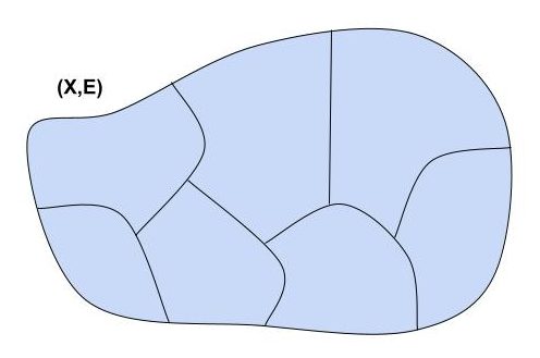
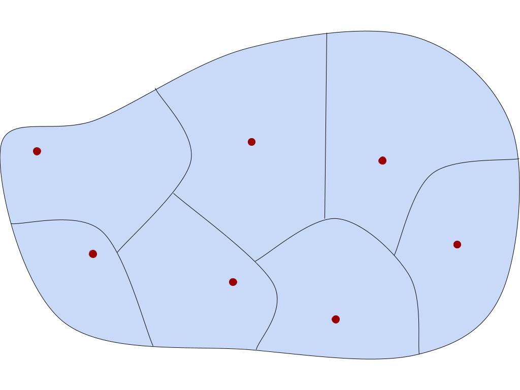
In the real world, classification is often vague. In math, it can be made a bit more precise through the notion of an equivalence relation. An equivalence relation can be thought of in two ways. First, concretely, it’s a way to “carve up” a set, partitioning it into disjoint pieces called equivalence classes. Every element x of the original set appears in exactly one equivalence class, which is referred to as [x].

More abstractly, an equivalence relation on a set X is a binary relation E on X satisfying three axioms:

Reflexivity: (∀x ∈ X) (x E x)
Symmetry: (∀x,y ∈ X) (x E y ⇒ y E x)
Transitivity: (∀x,y,z ∈ X) (x E y E z ⇒ x E z)

One can prove that any binary relation satisfying these three axioms yields a carving-up of X in the sense described above.

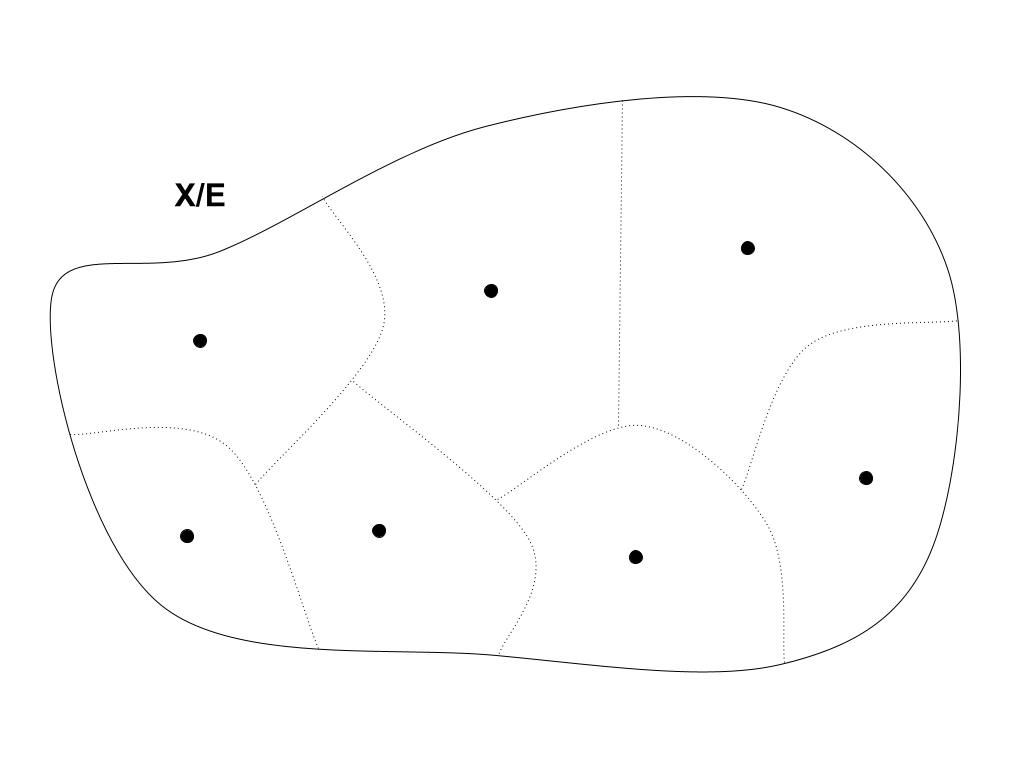
One thing that classification systems allow you to do is to coarse-grain the world, forgetting about the finer details and remembering only higher-order properties. Rather than think about my dog in particular, I can think about the class of all dogs, and treat this class as an object in its own right. Mathematically, this is called quotienting.

Quotienting is a very common mathematical move that appears wherever there are equivalence relations around. If E is an equivalence relation on a set X, then the quotient of X by E (written X/E) is just the set of all the equivalence classes.

X/E = { [x] | x ∈ X }

Quotienting can change structures in interesting and complicated ways. One of the most common examples is ℤ_n (the integers mod n), which we get by quotienting the integers ℤ by the “differs-by-n” equivalence relation:

x ~ y ⇔ |x – y| = n

For instance, in ℤ₅, the number 2 is identified with the equivalence class [2] = {…, -8, -3, 2, 7, 12, …}.

Equally common, the real numbers are often defined by quotienting. You start with the set of all Cauchy sequences of rational numbers, and consider the equivalence relation of “converging to one another” between sequences:

x ~ y ⇔ lim_n→∞ |x_n – y_n| = 0

A real number is defined to be an equivalence class of such sequences. This is a good example of coarse-graining in practice. You never really think of real numbers as sets of Cauchy sequences of rationals (outside of an analysis course). Once you quotient out by this equivalence relation, you forget about this “internal structure” and treat each real number as a primitive object. Similarly, in ℤ₅ you think of 2 as a primitive element, not an infinite set of integers.

Some classifications are harder than others

Let’s quickly recap the discussion in the last post.

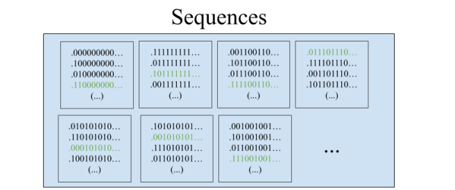
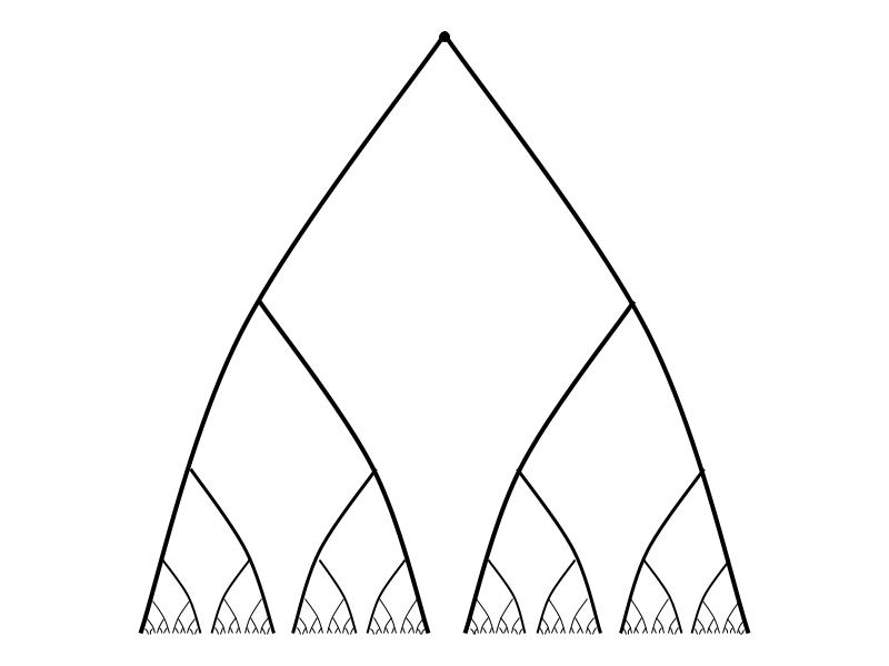
We began with an infinite group of prisoners whose freedom rested on their ability to pick representatives from a particular equivalence relation on Cantor space, 2^ℕ. Cantor space can be thought of in many ways. In our case, it’s the space of all ways of assigning black and white hats to the lineup. It’s also the space of all infinite binary sequences, or equivalently all functions from ℕ to {0,1}. And it can be visualized as the infinite paths through the complete infinite binary tree.

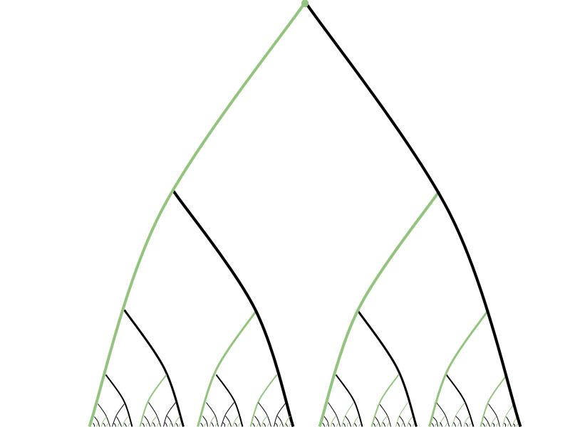
The equivalence relation the prisoners found themselves stuck with was the “eventually agrees” relation, E₀, defined by:

x E₀ y ⇔ (∃n ∈ ℕ) (∀m > n) (x_m = y_m)

For instance, here’s what the equivalence class of the all-zeros sequence 000… looks like:

The prisoners had to find some way of agreeing on a choice of representative from each equivalence class. There’s actually a few different ways to formalize this idea: transversals, selectors, and reductions.

A transversal of an equivalence relation E on X is a subset A ⊆ X which intersects each E-class exactly once.

(∀C ∈ X/E) (|A ∩ C| = 1)

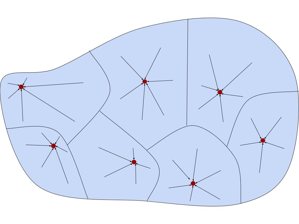
A selector for an equivalence relation E on X is a function f: X → X which takes the elements of an equivalence class C to the representative element for C.

(∀x ∈ X) (f(x) ∈ [x]_E) and (∀x,y ∈ X) (xEy ⇒ f(x) = f(y))

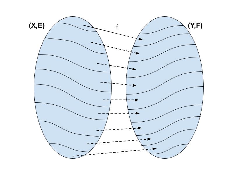
And finally (and most importantly) there’s the idea of a reduction. This idea is significantly more general than the previous two, and will play a big role in the upcoming posts. First, the formal definition:

Given two sets X,Y and equivalence relations E (on X) and F (on Y),
a reduction of E to F is a function f: X → Y such that
(∀x, x’ ∈ X) (x E x’ ⟺ f(x) F f(x’))

If such a function exists, we say that E is reducible to F and write E ≤ F.

Informally, reducibility measures the relative complexity of equivalence relations. If E ≤ F, then E is “simpler” or “easier. to compute” than F. For instance, if we want to check if two elements x and x’ are E-related, we can instead check if f(x) and f(x’) are F-related. Thus if we had an oracle for F then we could figure out E (using f).

A special case of reduction is where F is just the identity relation =_Y on Y, in which case we have:

xEx’ if and only if f(x) = f(x’)

Now, if we’re allowed to use any function f whatsoever, then this notion of reducibility ends up not being not so interesting. For instance, we can reduce any equivalence relation to equality by choosing Y = X/E and defining f(x) = [x]_E. More generally, reducibility with arbitrary functions turns out to just be a matter of comparing the cardinalities of the quotients. Thus we shift our focus from arbitrary functions to definable functions, in the sense of Borel.

In the last post we talked about Borel subsets of a space, not functions. But a function can be identified with its graph and treated as a subset of X × Y. So f: X → Y is Borel if and only if it is Borel as a subset of X × Y. Borel relations are defined similarly.

(Reminder: the Borel sets in a topological space X are just the sets you can construct out of open sets through countable unions, intersections, and complements. Equivalently, they’re the sets definable in countable propositional logic, with atomic propositions interpreted as defining the basic open sets.)

(Notice that we’re taking advantage of the relationship between definability and topology: if X and Y are both topological spaces, then the product X × Y already has a canonical “product topology”, generated by products of open sets in X and Y. So once we know how to interpret the atomic propositions in X and in Y, we can automatically interpret atomic propositions in X × Y.)

We’ve finally arrived at the central concept: Borel reducibility or definable reducibility.

Given two topological spaces X,Y and equivalence relations E (on X) and F (on Y),
a Borel reduction of E to F is a Borel function f: X → Y such that
(∀x, x’ ∈ X) (x E x’ ⟺ f(x) F f(x’))

If such a function exists, we say that E is Borel reducible to F and write E ≤_B F.

Classifying classifications

Let me now get to the punchline.

We carve up the mathematical universe by defining equivalence relations on the sets we’re interested in. When these sets are topological spaces, we can compare these equivalence relations through the relationship of Borel reducibility. At the end of the last post, I told you that there was no Borel transversal of E₀. By the same token, there is no Borel reduction of E₀ to the identity relation on Cantor space. “Eventual equality” is a strictly more complicated notion than “equality”.

This might not sound very surprising. Of course eventual equality is more complicated than equality, it has an extra word in its name! But it turns out that lots of complicated-looking equivalence relations are Borel reducible to the equality relation. Such equivalence relations are called smooth or concretely classifiable. For example, the relationship of “similarity” between square matrices (intuitively, two matrices are similar if they represent the same linear transformation but in different bases) turns out to be smooth.

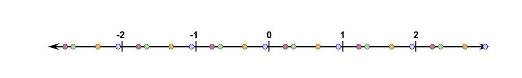
E is smooth if and only if there’s a Borel reduction E ≤_B =_ℝ

(Notice that I defined it here in terms of identity on ℝ rather than 2^ℕ. Not all identity relations are of equal complexity, but these two are. We’ll see that for many purposes ℝ and 2^ℕ are interchangeable.)

The smooth equivalence relations are the simplest ones out there. If E is smooth, then there’s some definable way to assign a different real number to each class. We can begin to draw a picture of the Borel reducibility hierarchy:

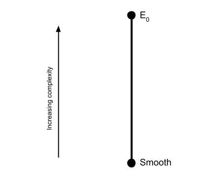
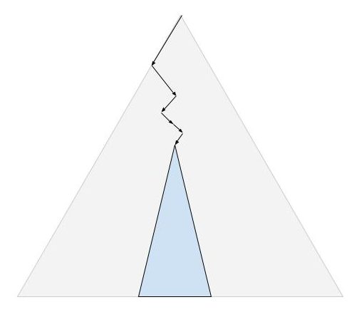
Natural questions immediately arise. Are there any equivalence relations strictly between smooth and E₀? (No.) Are there equivalence relations above E₀? (Yes, many.) Is there a most complex equivalence relation? (No, for any equivalence relation there’s a strictly harder one.) Are there equivalence relations of incomparable complexity? (Yes, in fact there’s uncountably many such equivalence relations!)

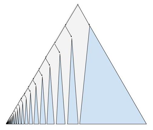
The Borel reducibility hierarchy for equivalence relations is a relatively recent discovery in the history of mathematics. It’s only about twenty years old. As such, there are many open questions about its structure. For instance, at the time of writing it’s unknown whether there’s exactly one class directly above E₀. There could be multiple incomparable classes directly above E₀, or it could be that for any equivalence relation E above E₀, there’s another one strictly in between E₀ and E.

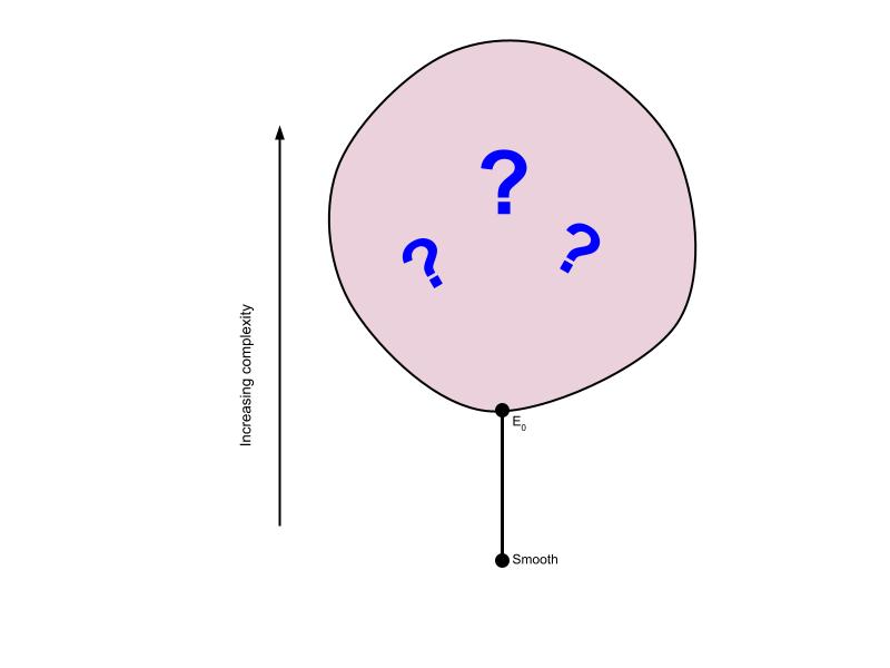
The big balloon represents the unknown territory waiting to be explored. But one thing that is clear at this point is that the internal structure of this balloon is very rich. In upcoming posts I hope to describe some of what we do know about it, and describe some recent attempts to probe its structure using techniques in model theory and infinitary first-order logic.

Choosing things is hard: infinite hats, definability, and topology

September 21, 2023September 25, 2023 ~ squarishbracket ~ Leave a comment

A hat puzzle

Infinitely many prisoners are assembled in a line as pictured. Each knows their place in the line. Each wears either a black or white hat, and each can only see the hats in front of them. Starting from the back of the line, each prisoner has to guess the color of their own hat. The prisoners were allowed to coordinate before the hats were assigned, but now no communication is allowed. Even the guesses must be silently submitted.

If only finitely many prisoners guess wrong, then everybody goes free. Can they succeed?

(Pause for thought.)

Amazingly, yes! Here’s the strategy:

Label white hats as 1 and black as 0. Then an assignment of hats becomes an infinite binary sequence, i.e. an element of 2^ℕ. Define an equivalence relation called E₀ on 2^ℕ as follows:

x E₀ y if and only if (∃n ∈ ℕ) (∀m > n) (x_m = y_m)
“x and y eventually agree”

When the prisoners meet up beforehand, they coordinate by agreeing on a choice of one representative from each class.

Once they’re in the room, every prisoner can see all but a finite number of hats. So they all know exactly which equivalence class they’re in. Now each prisoner guesses as if they were in the representative sequence from this class. Since the actual sequence and the representative sequence eventually agree, the prisoners’ guesses eventually agree with reality, and so they go free!

Making choices is hard

I talked about this puzzle a few years ago in this post. Several commenters balked at the solution and said something like: “but there are uncountably many equivalence classes, so therefore the prisoners need to be able to coordinate on uncountably many representatives. Surely this is unreasonable!”

I think that uncountably many representatives is not what’s at issue here. Consider the equivalence relation on the reals defined by:

x ~_ℤ y if and only if x – y ∈ ℤ.

Here we also have uncountably many equivalence classes, but the prisoners could easily come to an agreement on which representative to pick. They could for instance agree to choose the unique representative which lies in the interval [0,1). Here the prisoners are able to coordinate on uncountably many representatives, simply by agreeing on a function (f(x) = x mod 1) which takes each real to the representative for its class. A function f like this is called a reduction of ~_ℤ to =_ℝ, as it converts the problem of deciding x ~_ℤ y into the problem of deciding if two real numbers are equal (in particular, f(x) =_ℝ f(y)).

Now, is there a function f from 2^ℕ to 2^ℕ that takes an infinite binary sequence to the representative sequence for its class? That is, is there a reduction of E₀ to the identity relation on 2^ℕ? Sure! Each E₀-class C is non-empty, so we can “make a choice” of any element γ_C ∈ C. Then set f(x) = γ_[x], where [x] denotes the equivalence class of x.

I highlighted the key phrase in the above definition: make a choice. I said that we could choose an element from each class, but didn’t tell you how. And this is a problem for the prisoners! For them to all agree on the function’s values, they must be able to communicate how this choice is made to each other.

In the case of the equivalence relation ~_ℤ, we were able to find a precise recipe for choosing representatives, namely the definition of the function (x ↦ x mod 1). But can the prisoners find a precise recipe for choosing representatives for the E₀-classes?

That is, is there a definable function that reduces E₀ to =_ℝ? Well, what exactly is definability?

What is definability?

A major theme of descriptive set theory is the following identification, which I’d like to try to motivate:

DEFINABLE = BOREL

A definition is a syntactic thing. It’s a sentence with a free variable, like “x is the 15th digit in the decimal expansion of π” or “f is the identity function on ℝ”. To precisely state what definability is, we must specify a formal language to work in. The simplest logical language is that given by propositional logic. Here we begin with an alphabet, a countable set of basic atomic propositions, and build all other sentences through finite conjunctions, disjunctions, and negation.

Returning to our puzzle, we were interested in describing 2^ℕ and its subsets. We want our atomic propositions to represent easily definable subsets of 2^ℕ, or equivalently, simple properties of infinite binary sequences. A natural choice for these basic atomic properties is P_nm = “x’s nth bit is m”, interpreted as defining the set {x ∈ 2^ℕ | x’s nth bit is m}. Translated back to prisoners and hats, these are sentences like “Prisoner 35 is wearing a black hat” or “Prisoner 15 is wearing a white hat”. Intuitively, everything that can be said about infinite binary sequences, should be in principle expressible just in terms of sentences like these.

With finite conjunctions, disjunctions, and negation, we can define sets like {x ∈ 2^ℕ | x starts with 010110} and {x ∈ 2^ℕ | x’s first two bits agree}. Identifying 0 with “left” and 1 with “right”, we can draw these sets as subsets of the infinite binary tree:

How about a set like {x ∈ 2^ℕ | x contains at least one 1}?

What we want is a proposition like “x’s first bit is 0 or x’s second bit is 0 or …”, i.e.

(P₀₀ ∨ P₁₀ ∨ P₂₀ ∨ …), or \/_n∈ℕ P_n,0

What we need is the ability to take countably infinite conjunctions and disjunctions. Ordinary propositional logic doesn’t allow this. So we graduate to countable propositional logic. In other words, we expand the syntax by closing it under countable conjunctions and disjunctions:

For any countable collection of sentences {φ_n | n ∈ ℕ},
/\_nφ_n and \/_nφ_n are also sentences

On the semantic side, our collection of definable sets is now closed under countable unions, intersections, and negations. For the measure theorist, this is a familiar object: we’ve just defined a sigma-algebra!

(Technical note: when we say “closed under countable unions and intersections”, we also include empty unions and intersections, which correspond to ∅ and X, respectively. For notational convenience, we introduce the symbols ⊥ and ⊤ into our syntax, thought of as the atomic propositions “False” and “True”.)

In general there are many different sigma algebras you can put on a set, corresponding to different choices of the atomic propositions. But when our set is also a topological space, as in ℝ and 2^ℕ, there’s a natural choice of sigma-algebra, called the Borel sigma-algebra. Here we take our atomic propositions to define the basic (or sub-basic) open sets. Then the Borel sets are all the sets constructible through countable unions and intersections from basic opens, or equivalently, the sets definable in countable propositional logic.

In 2^ℕ the topology is generated by sets of the form

{x ∈ 2^ℕ | x’s nth bit is m} for any n, m ∈ ℕ,

which are the same as our earlier P_mn.

How about in ℝ? Here the topology is generated by basic sets of the form

(a,b) = {x ∈ ℝ | a < x < b} for any a, b ∈ ℚ

So we choose our atomic propositions accordingly: for any two rationals a,b, we have an atomic proposition P_ab, which we interpret as “a < x < b”.

Let’s pause to recall how we got here. We began by trying to define “definability”, and have found that there’s a natural way to interpret countable propositional logic through Borel sigma algebras on topological spaces. We have an atomic proposition for each (sub-)basic open set, and every set is defined by some countable propositional sentence. As we vary our interpretation of the atomic propositions, we move between different topological spaces.

The question “can the prisoners coordinate on a strategy?” has now taken on a definite form: “is there a Borel subset of 2^ℕ that picks exactly one element from each equivalence class?” And it turns out that the answer is no! For the prisoners to coordinate on a choice function, they need more syntactic resources at hand than countable propositional logic.

(To be continued…)

Who would win in a fight, logic or computation?

August 31, 2020August 31, 2020 ~ squarishbracket ~ 1 Comment

Which paradigm is stronger? When I say logic here, I’ll be referring to standard formal theories like ZFC and Peano arithmetic. If one uses an expansive enough definition to include computability theory, then logic encompasses computation and wins by default.

If you read this post, you might immediately jump to the conclusion that logic is stronger. After all, we concluded that in first order Peano arithmetic one can unambiguously define not only the decidable sets, but the sets decidable with halting oracles, and those decidable with halting oracles for halting oracles, and so on forever. We saw that the Busy Beaver numbers, while undecidable, are definable by a Π₁ sentence. And Peano arithmetic is a relatively weak theory; much more is definable in a theory like ZFC!

On the other hand, remember that there’s a difference between what’s absolutely definable and what’s definable-relative-to-ℕ. A set of numbers is absolutely definable if there’s a sentence that is true of just those numbers in every model of PA. It’s definable-relative-to-ℕ if there’s a sentence that’s true of just those numbers in the standard model of PA (the natural numbers, ℕ). Definable-relative-to-ℕ is an unfair standard for the strength of PA, given that PA, and in general no first order system, is able to categorically define the natural numbers. On the other hand, absolute definability is the standard that meets the criterion of “unambiguous definition”. With an absolute definition, there’s no room for confusion about which mathematical structure is being discussed.

All those highly undecidable sets we discussed earlier were only definable-relative-to-ℕ. In terms of what PA is able to define absolutely, it’s limited to only the finite sets. Compare this to what sets of numbers can be decided by a Turing machine. Every finite set is decidable, plus many infinite sets, including the natural numbers!

This is the first example of computers winning out over formal logic in their expressive power. While no first order theory (and in general no theory in a logic with a sound and complete proof system) can categorically define the natural numbers, it’s incredibly simple to write a program that defines that set using the language of PA. In regex, it’s just “S*0”. And here’s a Python script that does the job:

def check(s):
    if s == '':
        return False
    elif s == ‘0’:
        return True
    elif s[0] == ’s’:
        return check(s[1:])
    else:
        return False

We don’t even need a Turing machine for this; we can build a simple finite state machine:

In general, the sets decidable by computer can be much more complicated and interesting than those absolutely definable by a first-order theory. While first-order theories like ZFC have “surrogates” for infinite sets of numbers (ω and its definable subsets), these surrogate sets include nonstandard elements in some models. As a result, ZFC may fail to prove some statements about these sets which hold true of ℕ but fail for nonstandard models. For instance, it may be that the Collatz conjecture is true of the natural numbers but can’t be proven from ZFC. This would be because ZFC’s surrogate for the set of natural numbers (i.e. ω) includes nonstandard elements in some models, and the Collatz conjecture may fail for some such nonstandard elements.

On top of that, by taking just the first Turing jump into uncomputability, computation with a halting oracle, we are able to prove the consistency of ZFC and PA. Since ZFC is recursively axiomatizable, there’s a program that runs forever listing out theorems, such that every theorem is output at some finite point. We can use this to produce a program that looks to see if “0 = 1” is a theorem of ZFC. If ZFC is consistent, then the program will search forever and never find this theorem. But if ZFC is not consistent, then the program will eventually find the theorem “0 = 1” and will terminate at that point. Now we just apply our halting oracle to this program! If ZFC is consistent, then the halting oracle tells us that the program doesn’t halt, in which case we return “True”. If ZFC is not consistent, then the halting oracle tells us that the program does halt, in which case we return “False”. And just like that, we’ve decided the truth value of Con(ZFC)!

The same type of argument applies to Con(PA), and Con(T) for any T that is recursively axiomatizable. If you’re not a big fan of ZFC but have some other favored system for mathematics, then so long as this system’s axioms can be recognized by a computer, its consistency can be determined by a halting oracle.

Some summary remarks.

On the one hand, there’s a very simple explanation for why logic appears over and over again to be weaker than computation: we only choose to study formal theories that are recursively axiomatizable and have computable inference rules. Of course we can’t do better than a computer using a logical theory that can be built into a computer! If on the other hand, we chose true arithmetic, the set of all first-order sentences of PA that are true of ℕ, to be our de jure theory of mathematics, then the theorems of mathematics could not be recursively enumerated by any Turing machine, or indeed any oracle machine below 0^(ω). So perhaps there’s nothing too mysterious here after all.

On the other hand, there is something very philosophically interesting about truths of mathematics that cannot be proven just using mathematics, but could be proven if it happened that our universe gave us access to an oracle for the halting problem. If a priori reasoning is thought to be captured by a formal system like ZFC, then it’s remarkable that there are facts about the a priori (like Con(ZFC)) that cannot possibly be established by a priori reasoning. Any consistency proof cannot be provided by a consistent system itself, and going outside to a stronger system whose consistency is more in doubt doesn’t help at all. The only possible way to learn the truth value of such statements is contingent; we can learn it if the universe contains some physical manifestation of a halting oracle!

A Self-Interpreting Book

August 23, 2020August 23, 2020 ~ squarishbracket ~ 3 Comments

A concept: a book that starts by assuming the understanding of the reader and using concepts freely, and as you go on it introduces a simple formal procedure for defining words. As you proceed, more and more words are defined in terms of the basic formal procedure, so that halfway through, half of the words being used are formally defined, and by the end the entire thing is formally defined. Once you’re read through the whole book, you can start it over and read from the beginning with no problem.

I just finished a set theory textbook that felt kind of like that. It started with the extremely sparse language of ZFC: first-order logic with a single non-logical symbol, ∈. So the alphabet of the formal language consisted of the following symbols: ∈ ( ) ∧ ∨ ¬ → ↔ ∀ ∃ x ‘. It could have even started with a sparser formal language if it was optimizing for alphabet economy: ∈ ( ∧ ¬ ∀ x ‘ would suffice. As time passed and you got through more of the book, more and more things were defined in terms of the alphabet of ZFC: subsets, ordered pairs, functions from one set to another, transitivity, partial orders, finiteness, natural numbers, order types, induction, recursion, countability, real numbers, and limits. By the last chapter it was breathtaking to read a sentence filled with complex concepts and realize that every single one of these concepts was ultimately grounded in this super simple formal language we started with, with a finitistic sound and complete system of rules for how to use each one.

But could it be possible to really fully define ALL the terms used by the end of the book? And even if it were, could the book be written in such a way as to allow an alien that begins understanding nothing of your language to read it and, by the end, understand everything in the book? Even worse, what if the alien not only understands nothing of your language, but starts understanding nothing of the concepts involved? This might be a nonsensical notion; an alien that can read a book and do any level of sophisticated reasoning but doesn’t understand concepts like “and” and “or“.

One way that language is learned is by “pointing”: somebody asks me what a tree is, so I point to some examples of trees and some examples of non-trees, clarifying which is and which is not. It would be helpful if in this book we could point to simple concepts by means of interactive programs. So, for instance, an e-book where an alien reading the book encounters some exceedingly simple programs that they can experiment with, putting in inputs and seeing what results. So for instance, we might have a program that takes as input either 00, 01, 10, or 11, and outputs the ∧ operation applied to the two input digits. Nothing else would be allowed as inputs, so after playing with the program for a little bit you learn everything that it can do.

One feature of such a book would be that it would probably use nothing above first-order logical concepts. The reason is that the semantics of second-order logic cannot be captured by any sound and complete proof system, meaning that there’s no finitistic set of rules one could explain to an alien so that they know how to use the concepts involved correctly. Worse, the set of second-order tautologies is not even recursively enumerable (worse than the set of first-order tautologies, which is merely undecidable), so no amount of pointing-to-programs would suffice. First-order ZFC can define a lot, but can it define enough to write a book on what it can define?

On Self-Hating Theories of Arithmetic

June 15, 2020August 29, 2021 ~ squarishbracket ~ 6 Comments

Gödel’s second incompleteness theorem tells us that no (sufficiently powerful) consistent theory can prove the statement of its own consistency. But did you know that such a theory can prove the statement of its own inconsistency? A consistent theory that claims to be inconsistent is what I’ll call a self-hating theory.

My convention in what follows: ℕ refers to the real, true natural numbers, the set consisting of {0, 1, 2, 3, …} and nothing else. ω refers to the formal object that exists in a theory of arithmetic that is “supposed to be” ℕ, but (in first-order logic) cannot be guaranteed to be so.

When I write ℕ ⊨ ψ, I am saying that the sentence ψ is true of the natural numbers. When I write T ⊢ ψ (resp. T ⊬ ψ), I am saying that the sentence ψ can be (resp. can’t be) proven from the axioms of the theory T. And when I write T ⊨ ψ, I am saying that the axioms of T semantically entail the truth of ψ (or in other words, that ψ comes out true in all models of T). The next two paragraphs will give some necessary background on Gödel’s encoding, and then we’ll explore the tantalizing claims I started with.

Gödel’s breathtakingly awesome insight was that within any language that is expressive enough to talk about natural number arithmetic, one can encode sentences as numbers and talk about syntactic features of these sentences as properties of numbers. When a number n encodes a sentence ψ, we write n = ⟦ψ⟧. Then Gödel showed that you can have sentences talking about the provability of other sentences. (The next step, of course, was showing that you can have sentences talking about their own provability – sneaking in self-reference through the back door of any structure attempting to describe arithmetic.)

In particular, in any theory of natural number arithmetic T, one can write a sentence that on its surface appears to just be a statement about the properties of natural numbers, but when looked at through the lens of Gödel’s encoding, ends up actually encoding the sentence “T ⊢ ψ”. And this sentence is itself encoded as some natural number! So there’s a natural number n such that n = ⟦T ⊢ ψ⟧. It’s a short step from here to generating a sentence that encodes the statement of T’s own consistency. We merely need to encode the sentence “¬∃n (n = ⟦T ⊢ 0=1⟧)”, or in English, there’s no number n such that n encodes a proof of “0=1” from the axioms of T. In even plainer English, no number encodes a proof of contradiction from T (from which it follows that there IS no proof of contradiction from T, as any proof of contradiction would be represented by some number). We write this sentence as Con(T).

Okay, now we’re in a position to write the original claim of this post more formally. If a theory T is consistent, then ℕ ⊨ Con(T). And Gödel’s second incompleteness theorem tells us that if ℕ ⊨ Con(T), then T ⊬ Con(T). But if T doesn’t prove the sentence Con(T), then no contradiction can be derived by adding ¬Con(T) as an axiom! So (T + ¬Con(T)) is itself a consistent theory, i.e. ℕ ⊨ Con(T + ¬Con(T)). But hold on! (T + ¬Con(T)) can prove its own inconsistency! Why? Because (T + ¬Con(T)) ⊢ ¬Con(T), i.e. it proves that a contradiction can be derived from the axioms of T, and it also has as axioms every one of the axioms of T! So the same number that encodes a proof of the inconsistency of T, also counts as a proof of the inconsistency of (T + ¬Con(T))!

Summarizing this all:

ℕ ⊨ Con(T)
⇒
T ⊬ Con(T)
⇒
ℕ ⊨ Con(T + ¬Con(T)),
but
(T + ¬Con(T)) ⊢ ¬Con(T + ¬Con(T))

There we have it, a theory that is consistent but proves its own inconsistency!

Expressed another way:

T ⊢ ∃n (n = ⟦T ⊢ 0=1⟧),
but
T ⊬ 0=1

Ok, so believe it or not, a lot of the strangeness of this can be explained away by thinking about the implications of nonstandard models of arithmetic. One easy way to see this is to reflect on the fact that, as we saw above, “T is consistent” becomes in Gödel’s encoding, “There is no natural number n such that n encodes a proof of T’s inconsistency.” Or more precisely, “T is consistent” becomes “There is no natural number n such that n = ⟦T ⊢ 0=1⟧.”

Now, no first-order theory can pin down the natural numbers.

(I’ve written about this here and here.) I.e. no first order theory can express a quantification like “there is no natural number N such that …”. You can try, for sure, by defining some object ω and adding axioms to restrict its structure to look more and more like ℕ, but no matter how hard you try, no matter how many axioms you add, there will always be models of the theory in which ω ≠ ℕ. In particular, ω will be a strict superset of ℕ in all of these nonstandard models (ℕ ⊂ ω), so that ω contains all the naturals but also additional nonstandard numbers.

So now consider what happens when we try to quantify over the naturals by saying “∀x ∈ ω”. This quantifier inevitably ranges over ALL of the elements of ω in each model, so it also touches the nonstandard numbers in the nonstandard models. This means that the theory only semantically entails quantified statements that are true of all possible nonstandard numbers! (Remember, T ⊨ ψ means that ψ is true in ALL models of T.)

One nice consequence of this is that if T has a model in which ω = ℕ then in this model “∀x∈ω Φ(x)” is true only if Φ(x) is true of all natural numbers. By the completeness of first-order logic, this means that T can’t prove “∀x∈ω Φ(x)” unless it’s true of ℕ. This is reassuring; if T ⊢ ∀x∈ω Φ(x) and T has a model in which ω = ℕ, then ℕ ⊨ ∀x∈ω Φ(x).

But the implication doesn’t go the other way! ℕ ⊨ ∀x∈ω Φ(x) does not guarantee us that T ⊢ ∀x∈ω Φ(x), because T can only prove that which is true in EVERY model. So T can only prove “∀x∈ω Φ(x)” if Φ(x) is true of all the naturals and every nonstandard number in every model of T!

This is the reason that we don’t know for sure that if Goldbach’s conjecture is true of ℕ, then it’s provable in Peano arithmetic. On the face of it, this looks quite puzzling; Goldbach’s conjecture can be written as a first-order sentence and first-order logic is complete, so if it’s true then how could we possibly not prove it? The answer is hopefully clear enough now: Goldbach’s conjecture might be true of all of ℕ but false of some nonstandard models of Peano arithmetic (henceforth PA).

You might be thinking “Well if so, then we can just add Goldbach’s conjecture as an axiom to PA and get rid of those nonstandard models!” And you’re right, you will get rid of those nonstandard models. But you won’t get rid of all the nonstandard models in which Goldbach’s conjecture is true! You can keep adding as axioms statements that are true of ℕ but false of some nonstandard model, and as you do this you rule out more and more nonstandard models. At the end of this process (once your theory consists of literally all the first-order sentences that are true of ℕ), you will have created what is known as “True Arithmetic”: {ψ | ℕ ⊨ ψ}.

But guess what! At this point, have you finally ruled out all the nonstandard models? No! There’s still many many more (infinitely many, in fact! Nonstandard models of every cardinality! So many models that no cardinality is large enough to describe how many!) Pretty depressing, right? There are all these models that agree with ℕ on every first order sentence! But they are still not ℕ (most obviously because they contain numbers larger than 0, 1, 2, and all the rest of ℕ).

The nonstandard models of True Arithmetic are the models that are truly irremovable in any first-order theory of arithmetic. Any axiom you add to try to remove them will also remove ℕ as a model. And when you remove ℕ as a model, some pretty wacky stuff begins to happen.

Fully armed now with new knowledge of nonstandard numbers, let’s return to the statement I started with at the top of this post: there are consistent theories that prove their own inconsistency. The crucial point, the thing that explains this apparent paradox, is that all such theories lack ℕ as a model.

If you think about this for a minute, it should make sense why this must be the case. If a theory T is consistent, then the sentence “∀x∈ω (x ≠ ⟦T ⊢ 0 = 1⟧)” is true in a model where ω = ℕ. So if T has such a model, then T simply can’t prove its own inconsistency, as it’s actually not inconsistent and the model where ω = ℕ will be able to see that! And once more, T can only prove what’s true in all of its models.

Okay, so now supposing T is consistent (i.e. ℕ ⊨ Con(T)), by Gödel’s second incompleteness theorem, T cannot prove its own consistency. This means that (T + ¬Con(T)) is a consistent theory! But (T + ¬Con(T)) no longer has ℕ as a model. Why? Because ℕ ⊨ Con(T) and (T + ¬Con(T)) ⊨ ¬Con(T). So for any consistent theory T, (T + ¬Con(T)) only has nonstandard models. What does this mean about the things that T + ¬Con(T) proves? It means that they no longer have to be true of ℕ. So for instance, even though ℕ ⊨ Con(T + ¬Con(T)), (T + ¬Con(T)) might end up proving ¬Con(T + ¬Con(T)). And in fact, it does prove this! As we saw up at the top of this post, a moment’s examination will show that (T + ¬Con(T)) asserts as an axiom that a contradiction can be derived from the axioms of T, but also contains all the axioms of T! So by monotonicity, (T + ¬Con(T)) proves ¬Con(T + ¬Con(T)).

What do we say of this purported proof of contradiction from (T + ¬Con(T))? Well, we know for sure that it’s not a standard proof, one that would be accepted by a mathematician. I.e., it asserts that there’s some n in ω that encodes a proof of contradiction from (T + ¬Con(T)). But this n is not actually a natural number, it’s a nonstandard number. And nonstandards encode proofs only in the syntactical sense; a nonstandard proof is a proof according to Gödel’s arithmetic encoding, but Gödel’s arithmetic encoding only applies to natural numbers. So if we attempted to translate n, we’d find that the “proof” it encoded was actually nonsense all along: a fake proof that passes as acceptable by wearing the arithmetic guise of a real proof, but in actuality proves nothing whatsoever.

Summarizing:

In first order logic, every theory of arithmetic has nonstandard models that foil our attempts to prove all the truths of ℕ. Theories of arithmetic with ONLY nonstandard models and no standard model can prove things that don’t actually hold true of ℕ. In particular, since theories of arithmetic can encode statements about their own consistency, theories that don’t have ℕ as a model can prove their own inconsistency, even if they really are consistent.

So much for first order logic. What about

Second Order Logic?

As you might already know, second order logic is capable of ruling out all nonstandard models. There are second order theories that are categorical for ℕ. But there’s a large price tag for this achievement: second order logic has no sound and complete proof system!

Sigh. People sometimes talk about nature being tricky, trying to hide aspects of itself from us. Often you hear this in the context of discussions about quantum mechanics and black holes. But I think that the ultimate trickster is logic itself! Want a logic that’s sound and complete? Ok, but you’ll have to give up the expressive power to allow yourself to talk categorically about ℕ. Want to have a logic with the expressive power to talk about ℕ? Ok, but you’ll have to give up the possibility of a sound and complete proof system. The ultimate structure of ℕ remains shifty, slipping from our view as soon as we try to look closely enough at it.

Suppose that T is a second order theory that is categorical for ℕ. Then for every second-order sentence ψ that is true of ℕ, T ⊨ ψ. But we can’t make the leap from T ⊨ ψ to T ⊢ ψ without a complete proof system! So there will be semantic implications of T that cannot actually be proven from T.

In particular, suppose T is consistent. Then T ⊨ Con(T), but T ⊬ Con(T), by Gödel’s second. And since T ⊬ Con(T), (T + ¬Con(T)) is consistent. But since T ⊨ Con(T), (T + ¬Con(T)) ⊨ Con(T). So (T + ¬Con(T)) ⊨ Con(T) ∧ ¬Con(T)!

In other words, T + ¬Con(T) actually has no model! But it’s consistent! There are consistent second-order theories that are actually not logically possible – that semantically entail a contradiction and have no models. How’s that for trickiness?

Updated Introduction to Mathematical Logic

June 11, 2020 ~ squarishbracket ~ 1 Comment

I’ve noticed that some of my posts that have gotten the most hits are my introductions to mathematical logic. Overall, I’m pretty happy with that series of posts, though I think since then I’ve come up with clearer and more precise ways of talking about the primary distinctions: syntax, semantics, and proof systems.

A little while ago, I gave a talk on the subject of “true but unprovable” statements. The goal of the talk was just to explore this notion and explain what exactly it means to a logician. In the course of developing the talk, I ended up re-summarizing the basics of mathematical logic. I think this summary makes a good “companion piece” to my earlier introductory series, as well as being more standard in its presentation. The most important slide is this one:

Here’s the link to the full slideshow: True but Unprovable

And here you can look through it on this blog (but some of the formatting got a little wacky in the embedding process).

True but Unprovable from Rishi Banerjee

Finiteness can’t be captured in a sound, complete, finitary proof system

June 8, 2020June 8, 2020 ~ squarishbracket ~ 2 Comments

Consider the sentence “This blog has finitely many posts.” Do you understand what this sentence means? Then no set of rules (even infinite, even uncomputable!) can model your reasoning. This claim may sound shocking, but it can be justified on solid metamathematical grounds.

Another example: the sentence “There are finitely many planets in the universe.” You don’t have to think it’s true, you just have to think you understand what it means. What’s the common theme? It’s the notion of there being ‘finitely many’ of some class of objects. Let’s imagine building a language that has the expressive resources of first-order logic (which are quite modest), plus an additional quantifier F, whose semantics are given by the following rule: Fx φ(x) is satisfied by a model iff there are only finitely many objects in that model that satisfy φ(x).

It turns out that any language consisting of first order logic plus the quantifier F can’t be axiomatized in any sound, complete, and finitary proof system. Notice that effective enumerability of the rules of the proof system is not a requirement here! So long as the language is strong enough to express the semantics of {∧, ¬, ∀, F, variables x_n, and relations R_n}, no set of sentences and sentence-manipulation rules in that language will suffice to capture these semantics.

Here’s a proof: consider the first-order theory of Peano arithmetic. This theory has nonstandard models (as any theory of arithmetic must have in a logic that is compact). All of these nonstandard models have the following feature: that there are numbers that are larger than infinitely many numbers. Think about what this means: this is a common feature of all nonstandards, so if we could write a sentence to express this feature then we could rule them all out! This is where the quantifier F steps in. With F, we can write the following simple sentence and add it to PA as an axiom:

∀x Fy (y < x)

In English: every number has finitely many numbers less than it. And with that, we’ve ruled out all nonstandard models! So now we have a theory that is categorical for ℕ. And that’s a big deal, metamathematically speaking!

Why? Well, as I’ve talked about in a previous post, you can prove some pretty strong limitative results about any logic that can produce a theory that’s categorical for ℕ. In particular, if we can produce such a theory then its logic cannot be compact. Quick proof: suppose a set of sentences Σ models ℕ. Add to Σ a constant c and the axioms “c ≠ 0”, “c ≠ 1”, “c ≠ 2”, and so on, and call this new set Σ’. Every finite subset of Σ’ models ℕ. So by compactness, Σ’ has a model. But this model is nonstandard – it contains numbers that aren’t natural numbers. And since Σ is a subset of Σ’, any model of Σ’ is also a model of Σ.

So compactness implies that no theory is categorical for ℕ. But compactness follows from the following three properties: a sound and complete proof system (Σ ⊢ α if and only if Σ ⊨ α), and that all proofs are only finitely long (try expressing this property without F!). Quick proof: If a set of sentences is finitely satisfied, then every finite subset of it has a model (by definition), so no finite subset of it can be refuted (by soundness), so the entire set can’t be refuted (by finite proofs), so the entire set is satisfied (by completeness).

So soundness + completeness + finiteness ⇒ compactness ⇒ the existence of nonstandard models of arithmetic in any theory that models ℕ. Which means that the semantics of F cannot be captured in any sound, complete, and finite proof system!

Take your pick: either you don’t really understand the semantics of the “finitely many” quantifier F, or no set of rules (not even requiring this set to be finite or computable) can fully capture your reasoning in finite-length proofs.

More information about related extensions of first-order logic and their limitations can be found here. The result I describe here is a rephrasing of results discussed there.

The Continuum Hypothesis is False

June 3, 2020June 3, 2020 ~ squarishbracket ~ 5 Comments

Before I read this paper, I thought that the continuum hypothesis probably did not have a truth value, and that ZFC + CH and ZFC + ¬CH are systems that equally well capture what it means to be a set. Now I think that the continuum hypothesis is actually false, and that ZFC + CH would not be an adequate representation of our intuitive notion of sets.

The argument in the paper is not a formal proof of ¬CH. Instead, it’s a refutation of the following form: “The continuum hypothesis is equivalent in ZFC to this statement which is obviously false. So the continuum hypothesis must be false.”

So what is this obviously false statement? It is a claim that an event that happens with 100% probability is impossible. More exactly, for any function that assigns to each real number a countable set of real numbers, the claim is that it’s impossible for there exist two real numbers x and y such that x is not in the countable set assigned to y and y is not in the countable set assigned to x.

Why is this obviously false? Well, imagine throwing darts at the real line, so as to randomly select a real each time. If we throw one dart, there is a probability of zero that we would hit a natural number. Why? Because the cardinality of the naturals is less than the cardinality of the reals. By the same token, there is a probability of zero that our dart hits a rational number (as the rationals are also only countably large).

Now, if we throw a second dart, the probability that we hit a real number that’s some rational distance away from the first real number is also zero. Again, this is just because we’re considering a countable set of candidates from an uncountable set of possibilities. So by the same token, if we assign to the first dart ANY countable set of real numbers, then there is probability zero that the second dart lands within that countable set. And if we also assign a countable set of real numbers to the second dart, there is also probability zero that the first dart happened to fall within the countable set assigned to the second.

So, to summarize in more general terms: for any function f that maps each real number to a countable set of real numbers, a random choice of x and y will give us that x ∉ f(y) and y ∉ f(x) with 100% probability. Now, the statement that is equivalent to the falsity of the continuum hypothesis (i.e. the existence of cardinalities between |ω| and |𝒫(ω)|) is that it’s possible to find two real numbers x and y that are not in each others’ countable sets.

Notice how weak this is! By randomly choosing real numbers, we will end up with two that are not in each others’ countable sets with probability 100%. But we’re not even saying that the probability 100% event will always happen! We’re just saying that it’s POSSIBLE that it happens! I.e. imagine that by some miraculous coincidence it happens that the first two real numbers we choose are within each others’ countable sets (technically, only one of them needs to be in the other’s countable set). After all, probability-zero events do happen. Not a problem! Just pick two new real numbers! And if this fails, pick again!

Pretty cool right? Well, it gets even cooler. We just saw that from the statement “for any function f that maps reals to countable sets of reals, there exists x and y such that x ∉ f(y) and y ∉ f(x)”, you can prove that |𝒫(ω)| > |ω₁| (where the cardinality of ω₁ is by definition the next cardinality after ω). We can now consider THREE reals x, y, and z. Consider mappings from two real numbers to a countable set of reals. We can now state that for any such mapping, none of the three reals is in the countable set assigned to the others. And this entails that we can prove that |𝒫(ω)| > |ω₂|! In other words, we can prove that there are at least TWO cardinalities in between the reals and the naturals!

And for ANY n, if we take the statement that there are n reals such that none is inside the countable set mapped to by the others, then we can use this to prove that |𝒫(ω)| > |ω_n-1|. Notice: whatever n we choose, there’s still probability 100% that the n reals don’t “overlap” in this way! So for any n, we’re again only claiming that it’s possible for an event with 100% probability to happen. And if we accept this, then this entails that there’s not just a single cardinality between |ω| and |𝒫(ω)|. There’s definitely at least two. And at least three. And so on for ANY finite value of n. Which means that there are infinitely many cardinalities between the naturals and the reals!

Ok, this is a good point to stop reading if you don’t want to know the technical details of how EXACTLY to prove the result and are satisfied to just know what the result says. But if not, then read on! (The proof is actually really short and simple, though it relies on some background knowledge about ordinals.)

I’ll prove the result for n = 2. Suppose that |𝒫(ω)| = ℵ₁ = |ω₁|. Then by the axiom of choice, there’s some well-ordering of the reals of order type ω₁. Call this well-ordering <. We define f(x) to be {y | y ≤ x}. Notice that since ω₁ is the FIRST uncountable ordinal, f(x) is always a countable set, no matter what x is! Then, since for any two reals, x ≤ y or y ≤ x, this entails that for any two reals, x ∈ f(y) or y ∈ f(x).

And we’re done! We’ve shown that if the continuum hypothesis is true, then there exists a function f such that for any two reals, x ∈ f(y) or y ∈ f(x). So if we think that there is no such function, then we must deny the continuum hypothesis.

Kolmogorov Complexity, Undecidability, and Incompleteness

May 29, 2020July 11, 2020 ~ squarishbracket ~ Leave a comment

Fix some programming language. For any string x, we define K(x) (the Kolmogorov complexity of x) to be the bit length of the shortest program that outputs x and halts, when fed the empty string as input. I’m going to prove some neat results about Kolmogorov complexity.

K(x) ≤ |x|

Our first result: for every x, K(x) ≤ |x|. This is because in the worst case, you can always just literally have your program write out the string. (Technically, there might be a constant overhead, like writing “print()” in Python, but we will subtract out this constant overhead from our definition of K(x) so that the above equality holds.)

Most binary strings have high Kolmogorov complexity

In particular, at most 1/2^k of strings have K(x) < |x| – k

Half of all binary strings have K(x) < |x| – 1
A quarter have K(x) < |x| – 2
One eighth have K(x) < |x| – 3

Here’s the proof. Define A to be the set of all binary strings of length n with K(x) ≤ n – k. Define B to be the set of all binary strings of length n. So |A|/|B| is the proportion of all length-n strings with K(x) < n – k.

Now, |B| = 2ⁿ. And there’s an injection from A to programs of binary length < n – k. So |A| ≤ the number programs of binary length < n – k. But this is at most 2^n-k.

So |A|/|B| < 2^n-k/2ⁿ = 1/2^k.

This means that if we’re looking at strings of length 100, the proportion of them that have K(x) < 90 is at most 1/2¹⁰ = 1/1024 ≈ 0.1%. Said another way, more than 99.9% of length 100 strings have Kolmogorov complexity 90 or up (i.e. can only be compressed by at most 10 bits).

K(x) is uncomputable

There is no program that takes in a pair (x, k) and halts, outputting yes if K(x) = k and no if K(x) ≠ k. Let’s prove it.

Suppose that P is such a program. We use P to create a program Q that takes as input a number k and generates the first binary string y such that K(y) > k. Here’s how Q works: Enumerate all programs in lexicographic order (0, 1, 00, 01, 10, 11, 000, and so on). For each program x, apply P to check if K(x) = k. Output the first one for which the answer is yes.

Let’s give the name y to the output of Q on input k. Now, K(y) = k, because P says so. So the shortest program that outputs y has bit-length k. But notice that Q is also a program that outputs y! So the bit-length of Q has be at least k. But what is the bit-length of Q? Well, Q contains P as a subroutine, and writing Q requires that you also write out k. So |Q| = |P| + |k| + c (c is some constant overhead). But |k| is just the number of bits required to write out the number k, which is at most log₂(k).

So, K(y) = k ≤ |Q| ≤ log₂(k) + |P| + c. And this identity must hold no matter WHAT k we choose. So it must be that for all k, k ≤ log₂(k) + some constant. But this can’t be true! After all, k – log₂(k) goes to infinity as k goes to infinity! Contradiction.

The uncomputability of Kolmogorov complexity allows us to easily prove some of the most important and fun results in theoretical computer science. First of all:

The halting problem is undecidable

In other words, there is no program that takes as input a program P and outputs whether P will halt when run on the empty string.

Proof: Suppose that H is such a program. We can design a program using H to compute Kolmogorov complexity. Here’s how we do it: On input (x, k), enumerate all programs in lexicographic order. On each program Q, apply H to check if Q halts on empty string as input. If so, move on to the next program. If not, run Q to see if it outputs x.

This finds the shortest program y that outputs x. Now just look at the bit-length of y! If y has length k, then output yes, and otherwise output no. So if we can solve the halting problem, then we can also compute Kolmogorov complexity. But we just showed that you can’t do this! Contradiction.

The Busy Beaver numbers are uncomputable

Define BB(N) to be the maximum number of steps run by a program with length N before halting (only looking at those length-N programs that do halt, of course).

We prove that there is no program that takes as input a number N and outputs BB(N). Suppose Y is such a program. We can use Y to design a program H that solves the halting problem. Here’s how:

H takes as input a program P, uses Y to evaluate BB(|P|), and then runs P for BB(|P|) steps. If P hasn’t halted by the end of this, then P will never halt. So H outputs yes if P halts after BB(|P|) steps, and otherwise outputs no. This solves the halting problem, but we just showed that you can’t do this! Contradiction.

The Busy Beaver numbers grow faster than every computable function.

This is actually a very similar proof to the last one. Suppose f(n) is a computable function that grows faster than BB(n). Use f(n) to construct g(n) = f(n) + c, such that g(n) > BB(n) for all n. g(n) is computable, so let Y be a program that computes g(n).

We can design a program H that solves the halting problem using Y. H takes as input a program P, then uses Y to evaluate g(|P|), then runs P for g(|P|) steps. If P hasn’t halted by the end of this, then P will never halt. So H outputs yes if P halts after g(|P|) steps, and otherwise outputs no.

This solves the halting problem, but we just proved you can’t do this! Contradiction.

Gödel’s first incompleteness theorem

Yes that’s right, we’re going to prove this using Kolmogorov complexity! The theorem says that there is no recursively enumerable proof system which is sound and complete for the natural numbers.

Suppose F is such a proof system. We can use F to design a program P that takes as input x and k and computes whether K(x) = k. First, translate K(x) = k into a question about natural numbers. Then run through every string s in our proof system, checking at each step if s is a valid proof in F of K(x) = k, or of K(x) ≠ k. If either one of these is true, terminate and return which one. Since F is sound and complete, this algorithm eventually terminates and tells us which is true.

So if F existed, then we could compute Kolmogorov complexity. But we can’t compute Kolmogorov complexity! Contradiction. So there can not be any recursively enumerable proof system which is sound and complete for the natural numbers.

There’s an upper bound on what Kolmogorov complexities we can prove a string to have.

The proof of this closely resembles G. G. Berry’s paradox of ‘the first natural number which cannot be named in less than a billion words’ [P. R.: But this sentence names the very number in 14 words!]… The version of Berry’s paradox that will do the trick is ‘that object having the shortest proof that its algorithmic information content is greater than a billion bits.
Chaitin (1982)

For any sound proof system F, there’s a number L such that F cannot prove that the Kolmogorov complexity of any specific string of bits is more than L.

Suppose not. Then there’s some proof system F that is sound for N, such that for any L, F can prove that K(x) = L for some x.

First we design a program P that takes as input L and outputs a string x such that K(x) = L. P searches through proofs in F until it finds a proof that K(x) = L for some x, and then outputs x. F can prove this for any L by assumption.

Okay, so for each L, P(L) gives an x such that K(x) = L. So the shortest program that outputs x must be at least length L. But P(L) is a program that outputs x. So it must be that |P(L)| < L. But |P(L)| = |P| + |L| + c ≤ |P| + log₂(L) + c (for the same reasons as before). So it must be that for all L, L < |P| + log₂(L) + c. But as L goes to ∞, (L – log₂(L)) goes to ∞. So we can find an L such that L > |P| + log₂(L) + c. Contradiction!

We just showed that there’s some L for which we cannot prove that the Kolmogorov complexity of any string is L. But notice that if we take this L and add one, L+1 will still be larger than |P| + log₂(L+1) + c. And same for L+2, L+3, and so on forever. So really we’ve shown that there’s an L for which we can’t prove that the Kolmogorov complexity of any string is L or greater.

John Baez calls this the “complexity barrier” and argues here that the L is probably not actually that big. He guesses that L is a few thousand digits long at most!

Meaning ain’t in the brain

April 26, 2020April 26, 2020 ~ squarishbracket ~ Leave a comment

I don’t know if there’s a name for the position that the meanings of our terms is pinned down by facts about the brain. The closest I know is semantic internalism, but a semantic internalist could think that meaning is pinned down by facts about qualia, which happen to not be facts about the brain. So I’ll make up a name for this position: call it physicalist semantic internalism.

Now, here’s an argument against physicalist semantic internalism that seems totally right to me.

What I mean by “second-order logical concepts” is the concepts of “and”, “or”, “not”, second-order quantifiers (“for all” and “for some”, ranging over not just objects but properties of objects), and the notions of functions, relations, and concepts.

The semantics of second order logic captures what I mean when I use second-order logical concepts.
No finite set of rules (and correspondingly no finite machine) can pin down the semantics of second order logic.
So no finite machine pins down what I mean when I use second-order logical concepts.
My brain is a finite machine.
So my brain does not pin down what I mean when I use second-order logical concepts.

And here’s another argument along similar lines:

The truth values of sentences about integers are determined by what we mean by integers.
The statement of the satisfiability of each Diophantine equation has a determinate truth value.
The statement of the satisfiability of each Diophantine equation is a statement about integers.
So the satisfiability of each Diophantine equation is fixed by what we mean by integers.
No finite machine can fix the satisfiability of each Diophantine equation.
Our brain is a finite machine.
So the meaning of integers is not contained in the brain.