Quantum Chess

Recently I’ve been thinking about both quantum mechanics and chess, and came up with a chess variant that blends the two. The difference between ordinary chess and quantum chess is the ability to put your pieces in superpositions. Here’s how it works!

Movement

There are five modes of movement you can choose between in quantum chess: Move, Split, Merge, Collapse, and Branchmove.

Modes 1 and 2 are for non-superposed pieces, and modes 3, 4, and 5 are for superposed pieces.

Mode 1: Move

This mode allows you to move just as you would in an ordinary chess game.

Mode 2: Split

In the split mode, you can choose a non-superposed piece and split it between two positions. You can’t choose a position that is occupied, even by a superposed piece, meaning that splitting moves can never be attacks.

One powerful strategy is to castle into a superposition, bringing out both rooks and forcing your opponent to gamble on which side of the board to stage an attack on.

Mode 3: Merge

In mode 3, you can merge the two branches of one of your superposed pieces, recombining them onto a square that’s accessible from both branches.

You can’t merge to a position that’s only accessible from one of the two branches, and you can’t merge onto a square that’s occupied by one of your own superposed pieces, but merge moves can be attacks.

Mode 4: Collapse

Mode 4 is the riskiest mode. In this mode, you choose one of your superposed pieces and collapse it. There are two possible outcomes: First, it might collapse to the position you clicked on. In this case, you now have a choice to either perform an ordinary move…

… or to split it into a new superposition.

But if you get unlucky, then it will collapse to the position you didn’t select. In this case, your turn is over and it goes to your opponent.

Mode 5: Branch Move

Finally, in a branch move, you relocate just one branch of the superposition, without collapsing the wave-function or affecting the other branch.

Piece Interactions

Attacking a Superposed Piece

What happens if you attack a superposed piece? The result is that the superposed piece collapses. If the piece collapses onto the square you attacked, then you capture it.

But if it collapses onto the other branch of the superposition, then it is safe, and your piece moves harmlessly into the square you just attacked.

This means that attacking a superposed piece is risky! It’s possible for your attack to backfire, resulting in the attacker being captured next turn by the same piece it attacked.

It’s also possible for a pawn to move diagonally without taking a piece, in a failed attack.

Line of Sight

Superposed pieces block the lines of sight of both your pieces and your opponent’s pieces. This allows you to defend your pieces or block open files, without fully committing to defensive positions.

Winning the Game

To win quantum chess, you must actually take the opponent’s king. Let’s see why it’s not enough to just get the opponent into a position that would ordinarily be checkmate:

It’s blue’s turn now, and things look pretty lost. But look what blue can do:

Now the red queen has to choose one of the two targets to attack, and there’s a 50% chance that she gets it wrong, in which case the blue king can freely take the red queen, turning a sure loss into a draw!

So how can red get a guaranteed win? It takes patience. Rather than trying to attack one of the two squares, the red queen can hang back and wait for a turn.

Now the blue king has two choices: leave superposition, after which they can be taken wherever they go. Or move one branch of the superposition, but any possible branch move results in a safe shot at the king with the queen. This can be repeated until the king is taken.

And that’s quantum chess! I’ve played several games with friends, and each time have noticed interesting and surprising strategies arising. Let me leave you with a quantum chess puzzle. Here’s a position I found myself in, playing red:

What do you think was my best move here?

On Self-Hating Theories of Arithmetic

Gödel’s second incompleteness theorem tells us that no (sufficiently powerful) consistent theory can prove the statement of its own consistency. But did you know that such a theory can prove the statement of its own inconsistency? A consistent theory that claims to be inconsistent is what I’ll call a self-hating theory.

My convention in what follows: ℕ refers to the real, true natural numbers, the set consisting of {0, 1, 2, 3, …} and nothing else. ω refers to the formal object that exists in a theory of arithmetic that is “supposed to be” ℕ, but (in first-order logic) cannot be guaranteed to be so.

When I write ℕ ⊨ ψ, I am saying that the sentence ψ is true of the natural numbers. When I write T ⊢ ψ (resp. T ⊬ ψ), I am saying that the sentence ψ can be (resp. can’t be) proven from the axioms of the theory T. And when I write T ⊨ ψ, I am saying that the axioms of T semantically entail the truth of ψ (or in other words, that ψ comes out true in all models of T). The next two paragraphs will give some necessary background on Gödel’s encoding, and then we’ll explore the tantalizing claims I started with.

Gödel’s breathtakingly awesome insight was that within any language that is expressive enough to talk about natural number arithmetic, one can encode sentences as numbers and talk about syntactic features of these sentences as properties of numbers. When a number n encodes a sentence ψ, we write n = ⟦ψ⟧. Then Gödel showed that you can have sentences talking about the provability of other sentences. (The next step, of course, was showing that you can have sentences talking about their own provability – sneaking in self-reference through the back door of any structure attempting to describe arithmetic.)

In particular, in any theory of natural number arithmetic T, one can write a sentence that on its surface appears to just be a statement about the properties of natural numbers, but when looked at through the lens of Gödel’s encoding, ends up actually encoding the sentence “T ⊢ ψ”. And this sentence is itself encoded as some natural number! So there’s a natural number n such that n = ⟦T ⊢ ψ⟧. It’s a short step from here to generating a sentence that encodes the statement of T’s own consistency. We merely need to encode the sentence “¬∃n (n = ⟦T ⊢ 0=1⟧)”, or in English, there’s no number n such that n encodes a proof of “0=1” from the axioms of T. In even plainer English, no number encodes a proof of contradiction from T (from which it follows that there IS no proof of contradiction from T, as any proof of contradiction would be represented by some number). We write this sentence as Con(T).

Okay, now we’re in a position to write the original claim of this post more formally. If a theory T is consistent, then ℕ ⊨ Con(T). And Gödel’s second incompleteness theorem tells us that if ℕ ⊨ Con(T), then T ⊬ Con(T). But if T doesn’t prove the sentence Con(T), then no contradiction can be derived by adding ¬Con(T) as an axiom! So (T + ¬Con(T)) is itself a consistent theory, i.e. ℕ ⊨ Con(T + ¬Con(T)). But hold on! (T + ¬Con(T)) can prove its own inconsistency! Why? Because (T + ¬Con(T)) ⊢ ¬Con(T), i.e. it proves that a contradiction can be derived from the axioms of T, and it also has as axioms every one of the axioms of T! So the same number that encodes a proof of the inconsistency of T, also counts as a proof of the inconsistency of (T + ¬Con(T))!

Summarizing this all:

ℕ ⊨ Con(T)

T ⊬ Con(T)

ℕ ⊨ Con(T + ¬Con(T)),
but
(T + ¬Con(T)) ⊢ ¬Con(T + ¬Con(T))

There we have it, a theory that is consistent but proves its own inconsistency!

Expressed another way:

T ⊢ ∃n (n = ⟦T ⊢ 0=1⟧),
but
T ⊬ 0=1

Ok, so believe it or not, a lot of the strangeness of this can be explained away by thinking about the implications of nonstandard models of arithmetic. One easy way to see this is to reflect on the fact that, as we saw above, “T is consistent” becomes in Gödel’s encoding, “There is no natural number n such that n encodes a proof of T’s inconsistency.” Or more precisely, “T is consistent” becomes “There is no natural number n such that n = ⟦T ⊢ 0=1⟧.”

Now, no first-order theory can pin down the natural numbers.

(I’ve written about this here and here.) I.e. no first order theory can express a quantification like “there is no natural number N such that …”. You can try, for sure, by defining some object ω and adding axioms to restrict its structure to look more and more like ℕ, but no matter how hard you try, no matter how many axioms you add, there will always be models of the theory in which ω ≠ ℕ. In particular, ω will be a strict superset of ℕ in all of these nonstandard models (ℕ ⊂ ω), so that ω contains all the naturals but also additional nonstandard numbers.

So now consider what happens when we try to quantify over the naturals by saying “∀x ∈ ω”. This quantifier inevitably ranges over ALL of the elements of ω in each model, so it also touches the nonstandard numbers in the nonstandard models. This means that the theory only semantically entails quantified statements that are true of all possible nonstandard numbers! (Remember, T ⊨ ψ means that ψ is true in ALL models of T.)

One nice consequence of this is that if T has a model in which ω = ℕ then in this model “∀x∈ω Φ(x)” is true only if Φ(x) is true of all natural numbers. By the completeness of first-order logic, this means that T can’t prove “∀x∈ω Φ(x)” unless it’s true of ℕ. This is reassuring; if T ⊢ ∀x∈ω Φ(x) and T has a model in which ω = ℕ, then ℕ ⊨ ∀x∈ω Φ(x).

But the implication doesn’t go the other way! ℕ ⊨ ∀x∈ω Φ(x) does not guarantee us that T ⊢ ∀x∈ω Φ(x), because T can only prove that which is true in EVERY model. So T can only prove “∀x∈ω Φ(x)” if Φ(x) is true of all the naturals and every nonstandard number in every model of T!

This is the reason that we don’t know for sure that if Goldbach’s conjecture is true of ℕ, then it’s provable in Peano arithmetic. On the face of it, this looks quite puzzling; Goldbach’s conjecture can be written as a first-order sentence and first-order logic is complete, so if it’s true then how could we possibly not prove it? The answer is hopefully clear enough now: Goldbach’s conjecture might be true of all of ℕ but false of some nonstandard models of Peano arithmetic (henceforth PA).

You might be thinking “Well if so, then we can just add Goldbach’s conjecture as an axiom to PA and get rid of those nonstandard models!” And you’re right, you will get rid of those nonstandard models. But you won’t get rid of all the nonstandard models in which Goldbach’s conjecture is true! You can keep adding as axioms statements that are true of ℕ but false of some nonstandard model, and as you do this you rule out more and more nonstandard models. At the end of this process (once your theory consists of literally all the first-order sentences that are true of ℕ), you will have created what is known as “True Arithmetic”: {ψ | ℕ ⊨ ψ}.

But guess what! At this point, have you finally ruled out all the nonstandard models? No! There’s still many many more (infinitely many, in fact! Nonstandard models of every cardinality! So many models that no cardinality is large enough to describe how many!) Pretty depressing, right? There are all these models that agree with ℕ on every first order sentence! But they are still not ℕ (most obviously because they contain numbers larger than 0, 1, 2, and all the rest of ℕ).

The nonstandard models of True Arithmetic are the models that are truly irremovable in any first-order theory of arithmetic. Any axiom you add to try to remove them will also remove ℕ as a model. And when you remove ℕ as a model, some pretty wacky stuff begins to happen.

Fully armed now with new knowledge of nonstandard numbers, let’s return to the statement I started with at the top of this post: there are consistent theories that prove their own inconsistency. The crucial point, the thing that explains this apparent paradox, is that all such theories lack ℕ as a model.

If you think about this for a minute, it should make sense why this must be the case. If a theory T is consistent, then the sentence “∀x∈ω (x ≠ ⟦T ⊢ 0 = 1⟧)” is true in a model where ω = ℕ. So if T has such a model, then T simply can’t prove its own inconsistency, as it’s actually not inconsistent and the model where ω = ℕ will be able to see that! And once more, T can only prove what’s true in all of its models.

Okay, so now supposing T is consistent (i.e. ℕ ⊨ Con(T)), by Gödel’s second incompleteness theorem, T cannot prove its own consistency. This means that (T + ¬Con(T)) is a consistent theory! But (T + ¬Con(T)) no longer has ℕ as a model. Why? Because ℕ ⊨ Con(T) and (T + ¬Con(T)) ⊨ ¬Con(T). So for any consistent theory T, (T + ¬Con(T)) only has nonstandard models. What does this mean about the things that T + ¬Con(T) proves? It means that they no longer have to be true of ℕ. So for instance, even though ℕ ⊨ Con(T + ¬Con(T)), (T + ¬Con(T)) might end up proving ¬Con(T + ¬Con(T)). And in fact, it does prove this! As we saw up at the top of this post, a moment’s examination will show that (T + ¬Con(T)) asserts as an axiom that a contradiction can be derived from the axioms of T, but also contains all the axioms of T! So by monotonicity, (T + ¬Con(T)) proves ¬Con(T + ¬Con(T)).

What do we say of this purported proof of contradiction from (T + ¬Con(T))? Well, we know for sure that it’s not a standard proof, one that would be accepted by a mathematician. I.e., it asserts that there’s some n in ω that encodes a proof of contradiction from (T + ¬Con(T)). But this n is not actually a natural number, it’s a nonstandard number. And nonstandards encode proofs only in the syntactical sense; a nonstandard proof is a proof according to Gödel’s arithmetic encoding, but Gödel’s arithmetic encoding only applies to natural numbers. So if we attempted to translate n, we’d find that the “proof” it encoded was actually nonsense all along: a fake proof that passes as acceptable by wearing the arithmetic guise of a real proof, but in actuality proves nothing whatsoever.

Summarizing:

In first order logic, every theory of arithmetic has nonstandard models that foil our attempts to prove all the truths of ℕ. Theories of arithmetic with ONLY nonstandard models and no standard model can prove things that don’t actually hold true of ℕ. In particular, since theories of arithmetic can encode statements about their own consistency, theories that don’t have ℕ as a model can prove their own inconsistency, even if they really are consistent.

So much for first order logic. What about

Second Order Logic?

As you might already know, second order logic is capable of ruling out all nonstandard models. There are second order theories that are categorical for ℕ. But there’s a large price tag for this achievement: second order logic has no sound and complete proof system!

Sigh. People sometimes talk about nature being tricky, trying to hide aspects of itself from us. Often you hear this in the context of discussions about quantum mechanics and black holes. But I think that the ultimate trickster is logic itself! Want a logic that’s sound and complete? Ok, but you’ll have to give up the expressive power to allow yourself to talk categorically about ℕ. Want to have a logic with the expressive power to talk about ℕ? Ok, but you’ll have to give up the possibility of a sound and complete proof system. The ultimate structure of ℕ remains shifty, slipping from our view as soon as we try to look closely enough at it.

Suppose that T is a second order theory that is categorical for ℕ. Then for every second-order sentence ψ that is true of ℕ, T ⊨ ψ. But we can’t make the leap from T ⊨ ψ to T ⊢ ψ without a complete proof system! So there will be semantic implications of T that cannot actually be proven from T.

In particular, suppose T is consistent. Then T ⊨ Con(T), but T ⊬ Con(T), by Gödel’s second. And since T ⊬ Con(T), (T + ¬Con(T)) is consistent. But since T ⊨ Con(T), (T + ¬Con(T)) ⊨ Con(T). So (T + ¬Con(T)) ⊨ Con(T) ∧ ¬Con(T)!

In other words, T + ¬Con(T) actually has no model! But it’s consistent! There are consistent second-order theories that are actually not logically possible – that semantically entail a contradiction and have no models. How’s that for trickiness?

Logic, Theism, and Boltzmann Brains: On Cognitively Unstable Beliefs

First case

Propositional logic accepts that the proposition A-A is necessarily true. This is called the law of the excluded middle. Intuitionist logic differs in that it denies this axiom.

Suppose that Joe is a believer in propositional logic (but also reserves some credence for intuitionist logic). Joe also believes a set of other propositions, whose conjunction we’ll call X, and has total certainty in X.

One day Joe discovers that a contradiction can be derived from X, in a proof that uses the law of the excluded middle. Since Joe is certain that X is true, he knows that X isn’t the problem, and instead it must be the law of the excluded middle. So Joe rejects the law of the excluded middle and becomes an intuitionist.

The problem is, as an intuitionist, Joe now no longer accepts the validity of the argument that starts at X and concludes -X! Why? Because it uses the law of the excluded middle, which he doesn’t accept.

Should Joe believe in propositional logic or intuitionism?

Second case

Karl is a theist. He isn’t absolutely certain that theism is correct, but holds a majority of his credence in theism (and the rest in atheism). Karl is also 100% certain in the following claim: “If atheism is true, then the concept of ‘evil’ is meaningless”, and believes that logically valid arguments cannot be made using meaningless concepts.

One day somebody presents the problem of evil to Karl, and he sees it as a crushing objection to theism. He realizes that theism, plus some other beliefs about evil that he’s 100% confident in, leads to a contradiction. So since he can’t deny these other beliefs, he is led to atheism.

The problem is, as an atheist, Karl no longer accepts the validity of the argument that starts at theism and concludes atheism! Why? Because the arguments rely on using the concept of ‘evil’, and he is now certain that this concept is meaningless, and thus cannot be used in logically valid arguments.

Should Karl be a theist or an atheist?

Third case

Tommy is a scientist, and she believes that her brain is reliable. By this, I mean that she trusts her ability to reason both deductively and inductively. However, she isn’t totally certain about this, and holds out a little credence for radical skepticism. She is also totally certain about the content of her experiences, though not its interpretation (i.e. if she sees red, she is 100% confident that she is experiencing red, although she isn’t necessarily certain about what in the external world is causing the experience).

One day Tommy discovers that reasoning deductively and inductively from her experiences leads her to a model of the world that entails that her brain is actually a quantum fluctuation blipping into existence outside the event hole of a black hole. She realizes that this means that with overwhelmingly high probability, her brain is not reliable and is just producing random noise uncorrelated with reality.

The problem is, if Tommy believes that her brain is not reliable, then she can no longer accept the validity of the argument that led her to this position! Why? Well, she no longer trusts her ability to reason deductively or inductively. So she can’t accept any argument, let alone this particular one.

What should Tommy believe?

— — —

How are these three cases similar and different? If you think that Joe should be an intuitionist, or Karl an atheist, then should Tommy believe herself to be a black hole brain? Because it turns out that many cosmologists have found themselves to be in a situation analogous to Case 3! (Link.) I have my own thoughts on this, but I won’t share them for now.

How will quantum computing impact the world?

A friend of mine recently showed me an essay series on quantum computers. These essays are fantastically well written and original, and I highly encourage anybody with the slightest interest in the topic to check them out. They are also interesting to read from a pedagogical perspective, as experiments in a new style of teaching (self-described as an “experimental mnemonic medium”).

There’s one particular part of the post which articulated the potential impact of quantum computing better than I’ve seen it articulated before. Reading it has made me update some of my opinions about the way that quantum computers will change the world, and so I want to post that section here with full credit to the original authors Michael Nielsen and Andy Matuschak. Seriously, go to the original post and read the whole thing! You won’t regret it.

No, really, what are quantum computers good for?

It’s comforting that we can always simulate a classical circuit – it means quantum computers aren’t slower than classical computers – but doesn’t answer the question of the last section: what problems are quantum computers good for? Can we find shortcuts that make them systematically faster than classical computers? It turns out there’s no general way known to do that. But there are some interesting classes of computation where quantum computers outperform classical.

Over the long term, I believe the most important use of quantum computers will be simulating other quantum systems. That may sound esoteric – why would anyone apart from a quantum physicist care about simulating quantum systems? But everybody in the future will (or, at least, will care about the consequences). The world is made up of quantum systems. Pharmaceutical companies employ thousands of chemists who synthesize molecules and characterize their properties. This is currently a very slow and painstaking process. In an ideal world they’d get the same information thousands or millions of times faster, by doing highly accurate computer simulations. And they’d get much more useful information, answering questions chemists can’t possibly hope to answer today. Unfortunately, classical computers are terrible at simulating quantum systems.

The reason classical computers are bad at simulating quantum systems isn’t difficult to understand. Suppose we have a molecule containing n atoms – for a small molecule, n may be 1, for a complex molecule it may be hundreds or thousands or even more. And suppose we think of each atom as a qubit (not true, but go with it): to describe the system we’d need 2^n different amplitudes, one amplitude for each bit computational basis state, e.g., |010011.

Of course, atoms aren’t qubits. They’re more complicated, and we need more amplitudes to describe them. Without getting into details, the rough scaling for an natom molecule is that we need k^n amplitudes, where . The value of k depends upon context – which aspects of the atom’s behavior are important. For generic quantum simulations k may be in the hundreds or more.

That’s a lot of amplitudes! Even for comparatively simple atoms and small values of n, it means the number of amplitudes will be in the trillions. And it rises very rapidly, doubling or more for each extra atom. If , then even natoms will require 100 million trillion amplitudes. That’s a lot of amplitudes for a pretty simple molecule.

The result is that simulating such systems is incredibly hard. Just storing the amplitudes requires mindboggling amounts of computer memory. Simulating how they change in time is even more challenging, involving immensely complicated updates to all the amplitudes.

Physicists and chemists have found some clever tricks for simplifying the situation. But even with those tricks simulating quantum systems on classical computers seems to be impractical, except for tiny molecules, or in special situations. The reason most educated people today don’t know simulating quantum systems is important is because classical computers are so bad at it that it’s never been practical to do. We’ve been living too early in history to understand how incredibly important quantum simulation really is.

That’s going to change over the coming century. Many of these problems will become vastly easier when we have scalable quantum computers, since quantum computers turn out to be fantastically well suited to simulating quantum systems. Instead of each extra simulated atom requiring a doubling (or more) in classical computer memory, a quantum computer will need just a small (and constant) number of extra qubits. One way of thinking of this is as a loose quantum corollary to Moore’s law:

The quantum corollary to Moore’s law: Assuming both quantum and classical computers double in capacity every few years, the size of the quantum system we can simulate scales linearly with time on the best available classical computers, and exponentially with time on the best available quantum computers.

In the long run, quantum computers will win, and win easily.

The punchline is that it’s reasonable to suspect that if we could simulate quantum systems easily, we could greatly speed up drug discovery, and the discovery of other new types of materials.

I will risk the ire of my (understandably) hype-averse colleagues and say bluntly what I believe the likely impact of quantum simulation will be: there’s at least a 50 percent chance quantum simulation will result in one or more multi-trillion dollar industries. And there’s at least a 30 percent chance it will completely change human civilization. The catch: I don’t mean in 5 years, or 10 years, or even 20 years. I’m talking more over 100 years. And I could be wrong.

What makes me suspect this may be so important?

For most of history we humans understood almost nothing about what matter is. That’s changed over the past century or so, as we’ve built an amazingly detailed understanding of matter. But while that understanding has grown, our ability to control matter has lagged. Essentially, we’ve relied on what nature accidentally provided for us. We’ve gotten somewhat better at doing things like synthesizing new chemical elements and new molecules, but our control is still very primitive.

We’re now in the early days of a transition where we go from having almost no control of matter to having almost complete control of matter. Matter will become programmable; it will be designable. This will be as big a transition in our understanding of matter as the move from mechanical computing devices to modern computers was for computing. What qualitatively new forms of matter will we create? I don’t know, but the ability to use quantum computers to simulate quantum systems will be an essential part of this burgeoning design science.

Quantum computing for the very curious
(Andy Matuschak and Michael Nielsen)

The EPR Paradox

The Paradox

I only recently realized how philosophical the original EPR paper was. It starts out by providing a sufficient condition for something to be an “element of reality”, and proceeds from there to try to show the incompleteness of quantum mechanics. Let’s walk through this argument here:

The EPR Reality Condition: If at time t we can know the value of a measurable quantity with certainty without in any way disturbing the system, then there is an element of reality corresponding to that measurable quantity at time t. (i.e. this is a sufficient condition for a measurable property of a system at some moment to be an element of the reality of that system at that moment:)

Example 1: If you measure an electron spin to be up in the z direction, then quantum mechanics tells you that you can predict with certainty that the spin in the z direction will up at any future measurement. Since you can predict this with certainty, there must be an aspect or reality corresponding to the electron z-spin after you have measured it to be up the first time.

Example 2: If you measure an electron spin to be up in the z-direction, then QM tells you that you cannot predict the result of measuring the spin in the x-direction at a later time. So the EPR reality condition does not entail that the x-spin is an element of the reality of this electron. It also doesn’t entail that the x-spin is NOT an element of the reality of this electron, because the EPR reality condition is merely a sufficient condition, not a necessary condition.

Now, what does the EPR reality condition have to say about two particles with entangled spins? Well, suppose the state of the system is initially

|Ψ> = (|↑↓ – |↓↑) / √2

This state has the unusual property that it has the same form no matter what basis you express it in. You can show for yourself that in the x-spin basis, the state is equal to

|Ψ> = (|→← – |←→) / √2

Now, suppose that you measure the first electron in the z-basis and find it to be up. If you do this, then you know with certainty that the other electron will also be measured to be up. This means that after measuring it in the z-basis, the EPR reality condition says that electron 2 has z-spin up as an element of reality.

What if you instead measure the first electron in the x-basis and find it to be right? Well, then the EPR reality condition will tell you that the electron 2 has x-spin right as an element of reality.

Okay, so we have two claims:

  1. That after measuring the z-spin of electron 1, electron 2 has a definite z-spin, and
  2. that after measuring the x-spin of electron 1, electron 2 has a definite x-spin.

But notice that these two claims are not necessarily inconsistent with the quantum formalism, since they refer to the state of the system after a particular measurement. What’s required to bring out a contradiction is a further assumption, namely the assumption of locality.

For our purposes here, locality just means that it’s possible to measure the spin of electron 1 in such a way as to not disturb the state of electron 2. This is a really weak assumption! It’s not saying that any time you measure the spin of electron 1, you will not have disturbed electron 2. It’s just saying that it’s possible in principle to set up a measurement of the first electron in such a way as to not disturb the second one. For instance, take electrons 1 and 2 to opposite sides of the galaxy, seal them away in totally closed off and causally isolated containers, and then measure electron 1. If you agree that this should not disturb electron 2, then you agree with the assumption of locality.

Now, with this additional assumption, Einstein Podolsky and Rosen realized that our earlier claims (1) and (2) suddenly come into conflict! Why? Because if it’s possible to measure the z-spin of electron 1 in a way that doesn’t disturb electron 2 at all, then electron 2 must have had a definite z-spin even before the measurement of electron 1!

And similarly, if it’s possible to measure the x-spin of electron 1 in a way that doesn’t disturb electron 2, then electron 2 must have had a definite x-spin before the first electron was measured!

What this amounts to is that our two claims become the following:

  1. Electron 2 has a definite z-spin at time t before the measurement.
  2. Electron 2 has a definite x-spin at time t before the measurement.

And these two claims are in direct conflict with quantum theory! Quantum mechanics refuses to assign a simultaneous x and z spin to an electron, since these are incompatible observables. This entails that if you buy into locality and the EPR reality condition, then you must believe that quantum mechanics is an incomplete description of nature, or in other words that there are elements of reality that can not described by quantum mechanics.

The Resolution(s)

Our argument rested on two premises: the EPR reality condition and locality. Its conclusion was that quantum mechanics was incomplete. So naturally, there are three possible paths you can take to respond: accept the conclusion, deny the second premise, or deny the first premise.

To accept the conclusion is to agree that quantum mechanics is incomplete. This is where hidden variable approaches fall, and was the path that Einstein dearly hoped would be vindicated. For complicated reasons that won’t be covered in this post, but which I talk about here, the prospects for any local realist hidden variables theory (which was what Einstein wanted) look pretty dim.

To deny the second premise is to say that in fact, measuring the spin of the first electron necessarily disturbs the state of the second electron, no matter how you set things up. This is in essence a denial of locality, since the two electrons can be time-like separated, meaning that this disturbance must have propagated faster than the speed of light. This is a pretty dramatic conclusion, but is what orthodox quantum mechanics in fact says. (It’s implied by the collapse postulate.)

To deny the first premise is to say that in fact there can be some cases in which you can predict with certainty a measurable property of a system, but where nonetheless there is no element of reality corresponding to this property. I believe that this is where Many-Worlds falls, since measurement of z-spin doesn’t result in an electron in an unambiguous z-spin state, but in a combined superposition of yourself, your measuring device, the electron, and the environment. Needless to say, in this complicated superposition there is no definite fact about the z-spin of the electron.

I’m a little unsure about where the right place to put psi-epistemic approaches like Quantum Bayesianism, which resolve the paradox by treating the wave function not as a description of reality, but solely as a description of our knowledge. In this way of looking at things, it’s not surprising that learning something about an electron at one place can instantly tell you something about an electron at a distant location. This does not imply any faster-than-light communication, because all that’s being described is the way that information-processing occurs in a rational agent’s brain.

Measurement without interaction in quantum mechanics

In front of you is a sealed box, which either contains nothing OR an incredibly powerful nuclear bomb, the explosion of which threatens to wipe out humanity permanently. Even worse, this bomb is incredibly unstable and will blow up at the slightest contact with a single photon. This means that anybody that opens the box to look inside and see if there really is a bomb in there would end up certainly activating it and destroying the world. We don’t have any way to deactivate the bomb, but we could maintain it in isolation for arbitrarily long, despite the prohibitive costs of totally sealing it off from all contact.

Now, for obvious reasons, it would be extremely useful to know whether or not the bomb is actually active. If it’s not, the world can breathe a sigh of relief and not worry about spending lots of money on keeping it sealed away. And if it is, we know that the money is worth spending.

The obvious problem is that any attempt to test whether there is a bomb inside will involve in some way interacting with the box’s contents. And as we know, any such interaction will cause the bomb to detonate! So it seems that we’re stuck in this unfortunate situation where we have to act in ignorance of the full details of the situation. Right?

Well, it turns out that there’s a clever way that you can use quantum mechanics to do an “interaction-free measurement” that extracts some information from the system without causing the bomb to explode!

To explain this quantum bomb tester, we have to first start with a simpler system, a classic quantum interferometer setup:

56290881_2206928609636330_5087758915278471168_n.jpg

At the start, a photon is fired from the laser on the left. This photon then hits a beam splitter, which deflects the path of the photon with probability 50% and otherwise does nothing. It turns out that a photon that gets deflected by the beam splitter will pick up a 90º phase, which corresponds to multiplying the state vector by exp(iπ/2) = i. Each path is then redirected to another beam splitter, and then detectors are aligned across the two possible trajectories.

What do we get? Well, let’s just go through the calculation:

56414061_2282711835312851_8013422270024253440_n.jpg

We get destructive interference, which results in all photons arriving at detector B.

Now, what happens if you add a detector along one of the two paths? It turns out that the interference vanishes, and you find half the photons at detector A and the other half at detector B! That’s pretty weird… the observed frequencies appear to depend on whether or not you look at which path the photon went on. But that’s not quite right, because it turns out that you still get the 50/50 statistics whenever you place anything along one path whose state is changed by the passing photon!

Huh, that’s interesting… it indicates that by just looking for a photon at detector A, we can get evidence as to whether or not something interacted with the photon on the way to the detector! If we see a photon show up at the detector, then we know that there must have been some device which changed in state along the bottom path. Maybe you can already see where we’re going with this…

56451973_332761710713682_6105714719035752448_n.jpg

We have to put the box in the bottom path in such a way that if the box is empty, then when the photon passes by, nothing will change about either its state or the state of the photon. And if the box contains the bomb, then it will function like a detector (where the detection corresponds to whether or not the bomb explodes)!

Now, assuming that the box is empty, we get the same result as above. Let’s calculate the result we get assuming that the box contains the bomb:

56500763_2329442300624457_6272255095300161536_n

Something really cool happens here! We find that if the bomb is active, there is a 25% chance that the photon arrives as A without the bomb exploding. And remember, the photon arriving at detector A allows us to conclude with certainty that the bomb is active! In other words, this setup gives us a 25% chance of safely extracting that information!

25% is not that good, you might object. But it sure is better than 0%! And in fact, it turns out that you can strengthen this result, using a more complicated interferometer setup to learn with certainty whether the bomb is active with an arbitrarily small chance of setting off the bomb!

There’s so many weird little things about quantum mechanics that defy our classical intuitions, and this “interaction-free measurements” is one of my new favorites.

Is the double slit experiment evidence that consciousness causes collapse?

No! No no no.

This might be surprising to those that know the basics of the double slit experiment. For those that don’t, very briefly:

A bunch of tiny particles are thrown one by one at a barrier with two thin slits in it, with a detector sitting on the other side. The pattern on the detector formed by the particles is an interference pattern, which appears to imply that each particle went through both slits in some sense, like a wave would do. Now, if you peek really closely at each slit to see which one each particle passes through, the results seem to change! The pattern on the detector is no longer an interference pattern, but instead looks like the pattern you’d classically expect from a particle passing through only one slit!

When you first learn about this strange dependence of the experimental results on, apparently, whether you’re looking at the system or not, it appears to be good evidence that your conscious observation is significant in some very deep sense. After all, observation appears to lead to fundamentally different behavior, collapsing the wave to a particle! Right?? This animation does a good job of explaining the experiment in a way that really pumps the intuition that consciousness matters:

(Fair warning, I find some aspects of this misleading and just plain factually wrong. I’m linking to it not as an endorsement, but so that you get the intuition behind the arguments I’m responding to in this post.)

The feeling that consciousness is playing an important role here is a fine intuition to have before you dive deep into the details of quantum mechanics. But now consider that the exact same behavior would be produced by a very simple process that is very clearly not a conscious observation. Namely, just put a single spin qubit at one of the slits in such a way that if the particle passes through that slit, it flips the spin upside down. Guess what you get? The exact same results as you got by peeking at the screen. You never need to look at the particle as it travels through the slits to the detector in order to collapse the wave-like behavior. Apparently a single qubit is sufficient to do this!

It turns out that what’s really going on here has nothing to do with the collapse of the wave function and everything to do with the phenomenon of decoherence. Decoherence is what happens when a quantum superposition becomes entangled with the degrees of freedom of its environment in such a way that the branches of the superposition end up orthogonal to each other. Interference can only occur between the different branches if they are not orthogonal, which means that decoherence is sufficient to destroy interference effects. This is all stuff that all interpretations of quantum mechanics agree on.

Once you know that decoherence destroys interference effects (which all interpretations of quantum mechanics agree on), and also that a conscious observing the state of a system is a process that results in extremely rapid and total decoherence (which everybody also agrees on), then the fact that observing the position of the particle causes interference effects to vanish becomes totally independent of the question of what causes wave function collapse. Whether or not consciousness causes collapse is 100% irrelevant to the results of the experiment, because regardless of which of these is true, quantum mechanics tells us to expect observation to result in the loss of interference!

This is why whether or not consciousness causes collapse has no real impact on what pattern shows up in the wall. All interpretations of quantum mechanics agree that decoherence is a thing that can happen, and decoherence is all that is required to explain the experimental results. The double slit experiment provides no evidence for consciousness causing collapse, but it also provides no evidence against it. It’s just irrelevant to the question! That said, however, given that people often hear the experiment presented in a way that makes it seem like evidence for consciousness causing collapse, hearing that qubits do the same thing should make them update downwards on this theory.

Decoherence is not wave function collapse

In the double slit experiment, particles travelling through a pair of thin slits exhibit wave-like behavior, forming an interference pattern where they land that indicates that the particles in some sense travelled through both slits.

54518134_416516682243379_7426065872885645312_n.jpg

Now, suppose that you place a single spin bit at the top slit, which starts off in the state |↑⟩ and flips to |↓⟩ iff a particle travels through the top slit. We fire off a single particle at a time, and then each time swap out that spin bit for a new spin bit that also starts off in the state |↑⟩. This serves as an extremely simple measuring device which encodes the information about which slit each particle went through.

Now what will you observe on the screen? It turns out that you’ll observe the classically expected distribution, which is a simple average over the two individual possibilities without any interference.

53857812_1014378252080175_1814900750900264960_n.jpg

Okay, so what happened? Remember that the first pattern we observed was the result of the particles being in a superposition over the two possible paths, and then interfering with each other on the way to the detector screen. So it looks like simply having one bit of information recording the path of the particle was sufficient to collapse the superposition! But wait! Doesn’t this mean that the “consciousness causes collapse” theory is wrong? The spin bit was apparently able to cause collapse all by itself, so assuming that it isn’t a conscious system, it looks like consciousness isn’t necessary for collapse! Theory disproved!

No. As you might be expecting, things are not this simple. For one thing, notice that this ALSO would prove as false any other theory of wave function collapse that doesn’t allow single bits to cause collapse (including anything about complex systems or macroscopic systems or complex information processing). We should be suspicious of any simple argument that claims to conclusively prove a significant proportion of experts wrong.

To see what’s going on here, let’s look at what happens if we don’t assume that the spin bit causes the wave function to collapse. Instead, we’ll just model it as becoming fully entangled with the path of the particle, so that the state evolution over time looks like the following:

54114815_2222391794691111_7588527245694599168_n

Now if we observe the particle’s position on the screen, the probability distribution we’ll observe is given by the Born rule. Assuming that we don’t observe the states of the spin bits, there are now two qualitatively indistinguishable branches of the wave function for each possible position on the screen. This means that the total probability for any given landing position will be given by the sum of the probabilities of each branch:

54432750_422324315183100_8833216438886989824_n-e1552873260955.jpg

But hold on! Our final result is identical to the classically expected result! We just get the probability of the particle getting to |j⟩ from |A⟩, multiplied by the probability of being at |A⟩ in the first place (50%), plus the probability of the particle going from |B⟩ to |j⟩ times the same 50% for the particle getting to |B⟩.

54220547_1042042785982437_8822680544807485440_n.jpg

In other words, our prediction is that we’d observe the classical pattern of a bunch of individual particles, each going through exactly one slit, with 50% going through the top slit and 50% through the bottom. The interference has vanished, even though we never assumed that the wave function collapsed!

What this shows is that wave function collapse is not required to get particle-like behavior. All that’s necessary is that the different branches of the superposition end up not interfering with each other. And all that’s necessary for that is environmental decoherence, which is exactly what we had with the single spin bit!

In other words, environmental decoherence is sufficient to produce the same type of behavior that we’d expect from wave function collapse. This is because interference will only occur between non-orthogonal branches of the wave function, and the branches become orthogonal upon decoherence (by definition). A particle can be in a superposition of multiple states but still act as if it has collapsed!

Now, maybe we want to say that the particle’s wave function is collapsed when its position is measured by the screen. But this isn’t necessary either! You could just say that the detector enters into a superposition and quickly decoheres, such that the different branches of the wave function (one for each possible detector state) very suddenly become orthogonal and can no longer interact. And then you could say that the collapse only really happens once a conscious being observes the detector! Or you could be a Many-Worlder and say that the collapse never happens (although then you’d have to figure out where the probabilities are coming from in the first place).

You might be tempted to say at this point: “Well, then all the different theories of wave function collapse are empirically equivalent! At least, the set of theories that say ‘wave function collapse = total decoherence + other necessary conditions possibly’. Since total decoherence removes all interference effects, the results of all experiments will be indistinguishable from the results predicted by saying that the wave function collapsed at some point!”

But hold on! This is forgetting a crucial fact: decoherence is reversible, while wave function collapse is not!!! 

Screen Shot 2019-03-17 at 8.21.51 PM
Pretty picture from doi: 10.1038/srep15330

Let’s say that you run the same setup before with the spin bit recording the information about which slit the particle went through, but then we destroy that information before it interacts with the environment in any way, therefore removing any traces of the measurement. Now the two branches of the wave function have “recohered,” meaning that what we’ll observe is back to the interference pattern! (There’s a VERY IMPORTANT caveat, which is that the time period during which we’re destroying the information stored in the spin bit must be before the particle hits the detector screen and the state of the screen couples to its environment, thus decohering with the record of which slit the particle went through).

If you’re a collapse purist that says that wave function collapse = total decoherence (i.e. orthogonality of the relevant branches of the wave function), then you’ll end up making the wrong prediction! Why? Well, because according to you, the wave function collapsed as soon as the information was recorded, so there was no “other branch of the wave function” to recohere with once the information was destroyed!

This has some pretty fantastic implications. Since IN PRINCIPLE even the type of decoherence that occurs when your brain registers an observation is reversible (after all, the Schrodinger equation is reversible), you could IN PRINCIPLE recohere after an observation, allowing the branches of the wave function to interfere with each other again. These are big “in principle”s, which is why I wrote them big. But if you could somehow do this, then the “Consciousness Causes Collapse” theory would give different predictions from Many-Worlds! If your final observation shows evidence of interference, then “consciousness causes collapse” is wrong, since apparently conscious observation is not sufficient to cause the other branches of the wave function to vanish. Otherwise, if you observe the classical pattern, then Many Worlds is wrong, since the observation indicates that the other branches of the wave function were gone for good and couldn’t come back to recohere.

This suggests a general way to IN PRINCIPLE test any theory of wave function collapse: Look at processes right beyond the threshold where the theory says wave functions collapse. Then implement whatever is required to reverse the physical process that you say causes collapse, thus recohering the branches of the wave function (if they still exist). Now look to see if any evidence of interference exists. If it does, then the theory is proven wrong. If it doesn’t, then it might be correct, and any theory of wave function collapse that demands a more stringent standard for collapse (including Many-Worlds, the most stringent of them all) is proven wrong.

On decoherence

Consider the following simple model of the double-slit experiment:

53215233_424625501621649_7989218325425029120_n

A particle starts out at |O⟩, then evolves via the Schrödinger equation into an equal superposition of being at position |A⟩ (the top slit) and being at position |B⟩ (the bottom slit).

53847892_379521639268098_6802808492659834880_n

To figure out what happens next, we need to define what would happen for a particle leaving from each individual slit. In general, we can describe each possibility as a particular superposition over the screen.

Since quantum mechanics is linear, the particle that started at |O⟩ will evolve as follows:

53847892_379521639268098_6802808492659834880_n
53847892_379521639268098_6802808492659834880_n-3.jpg

If we now look at any given position |j⟩ on the screen, the probability of observing the particle at this position can be calculated using the Born rule:

54435476_1877330259039769_997663582227267584_n-1.jpg

Notice that the first term is what you’d expect to get for the probability of a particle leaving |A⟩ being observed at position |j⟩ and the second term is the probability of a particle from |B⟩ being observed at |j⟩. The final two terms are called interference terms, and they give us the non-classical wave-like behavior that’s typical of these double-slit setups.

53695256_2103980996560637_2413894306092810240_n

Now, what we just imagined was a very idealized situation in which the only parts of the universe that are relevant to our calculation are the particle, the two slits and the detector. But in reality, as the particle is traveling to the detector, it’s likely going to be interacting with the environment. This interaction is probably going to be slightly different for a particle taking the path through |A⟩ than for a particle taking the path through |B⟩, and these differences end up being immensely important.

To capture the effects of the environment in our experimental setup, let’s add an “environment” term to all of our states. At time zero, when the particle is at the origin, we’ll say that the environment is in some state |ε0⟩. Now, as the particle traverses the path to |A⟩ or to |B⟩, the environment might change slightly, so we need to give two new labels for the state of the environment in each case. |εA⟩ will be our description for the state of the environment that would result if the particle traversed the path from |O⟩ to |A⟩, and |εB⟩ will be the label for the state of the environment resulting from the particle traveling from |O⟩ to |B⟩. Now, to describe our system, we need to take the tensor product of the vector for our particle’s state and the vector for the environment’s state:

54519367_308525316478932_3398984521884893184_n.jpg

Now, what is the probability of the particle being observed at position j? Well, there are two possible worlds in which the particle is observed at position j; one in which the environment is in state |εA⟩ and the other in which it’s in state |εB⟩. So the probability will just be the sum of the probabilities for each of these possibilities.

54211669_1846645752108144_5863174741849800704_n

This final equation gives us the general answer to the double slit experiment, no matter what the changes to the environment are. Notice that all that is relevant about the environment is the overlap term ⟨εAB⟩, which we’ll give a special name to:

54278294_2524715951075704_6933032674168668160_n

This term tells us how different the two possible end states for the environment look. If the overlap is zero, then the two environment states are completely orthogonal (corresponding to perfect decoherence of the initial superposition). If the overlap is one, then the environment states are identical.

53298673_333616094167211_1463267431869841408_n

And look what we get when we express the final probability in terms of this term!

53208725_1847238688713413_8130541857772929024_n-1.jpg

Perfect decoherence gives us classical probabilities, and perfect coherence gives us the ideal equation we found in the first part of the post! Anything in between allows the two states to interfere with each other to some limited degree, not behaving like totally separate branches of the wavefunction, nor like one single branch.

The problem with the many worlds interpretation of quantum mechanics

The Schrodinger equation is the formula that describes the dynamics of quantum systems – how small stuff behaves.

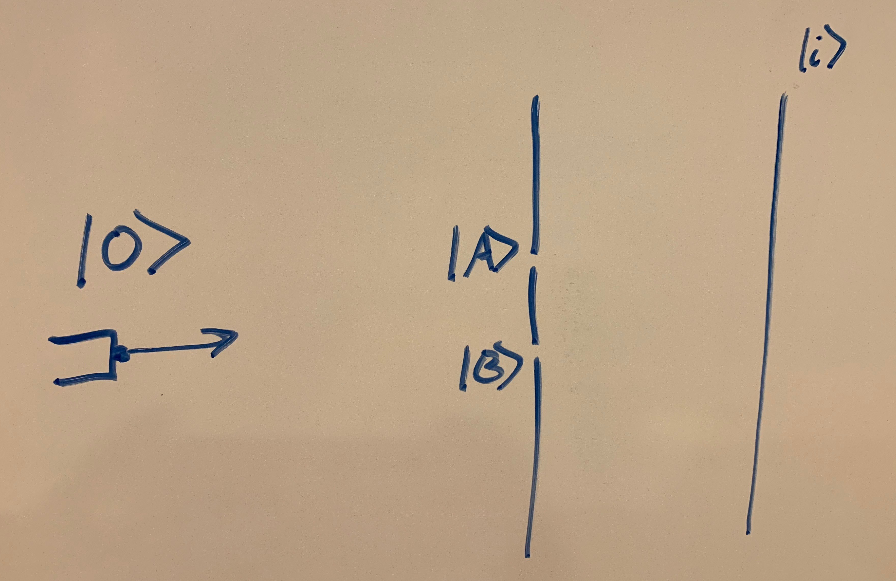
One fundamental feature of quantum mechanics that differentiates it from classical mechanics is the existence of something called superposition. In the same way that a particle can be in the state of “being at position A” and could also be in the state of “being at position B”, there’s a weird additional possibility that the particle is in the state of “being in a superposition of being at position A and being at position B”. It’s necessary to introduce a new word for this type of state, since it’s not quite like anything we are used to thinking about.

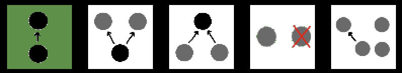
Now, people often talk about a particle in a superposition of states as being in both states at once, but this is not technically correct. The behavior of a particle in a superposition of positions is not the behavior you’d expect from a particle that was at both positions at once. Suppose you sent a stream of small particles towards each position and looked to see if either one was deflected by the presence of a particle at that location. You would always find that exactly one of the streams was deflected. Never would you observe the particle having been in both positions, deflecting both streams.

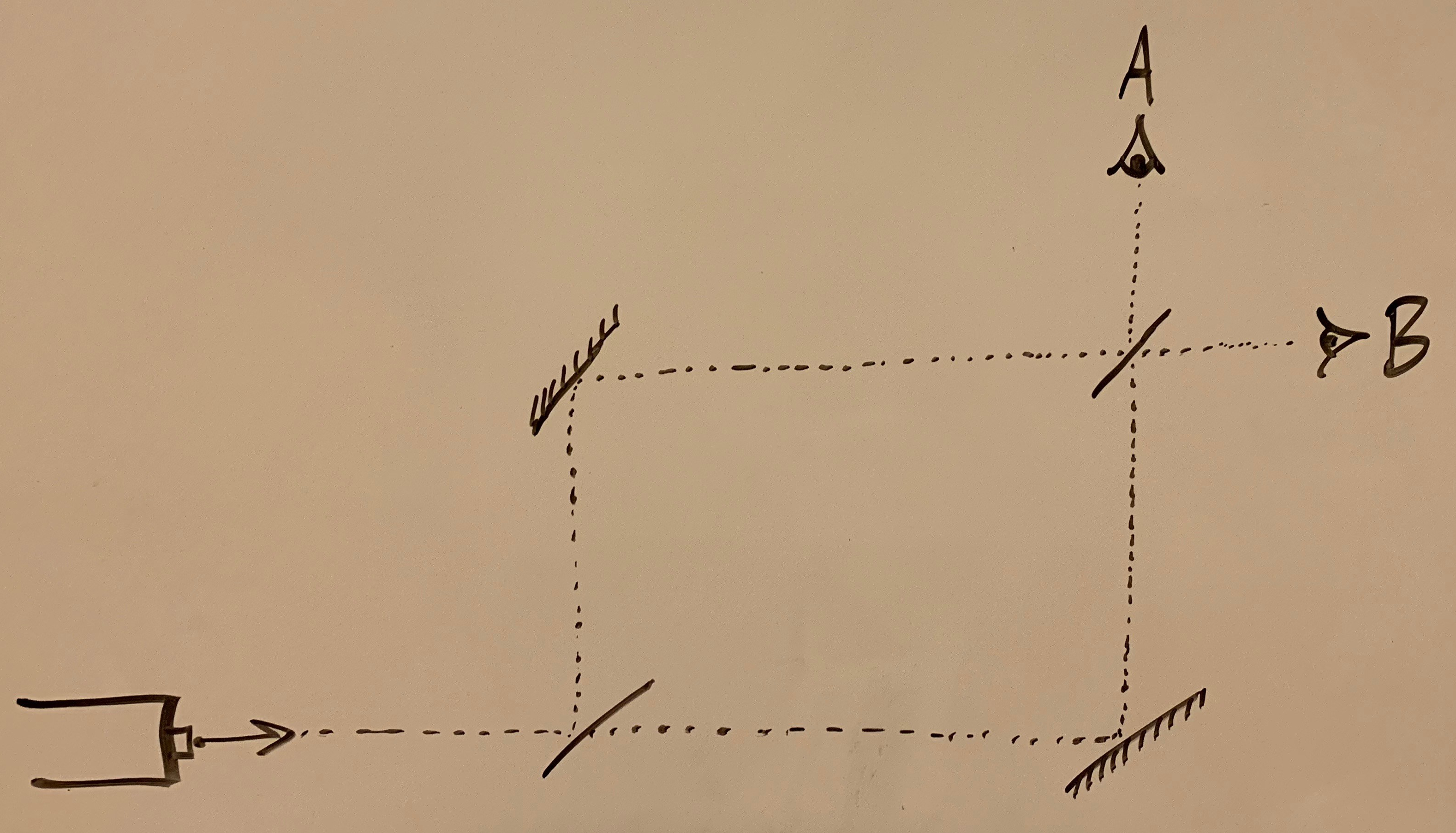
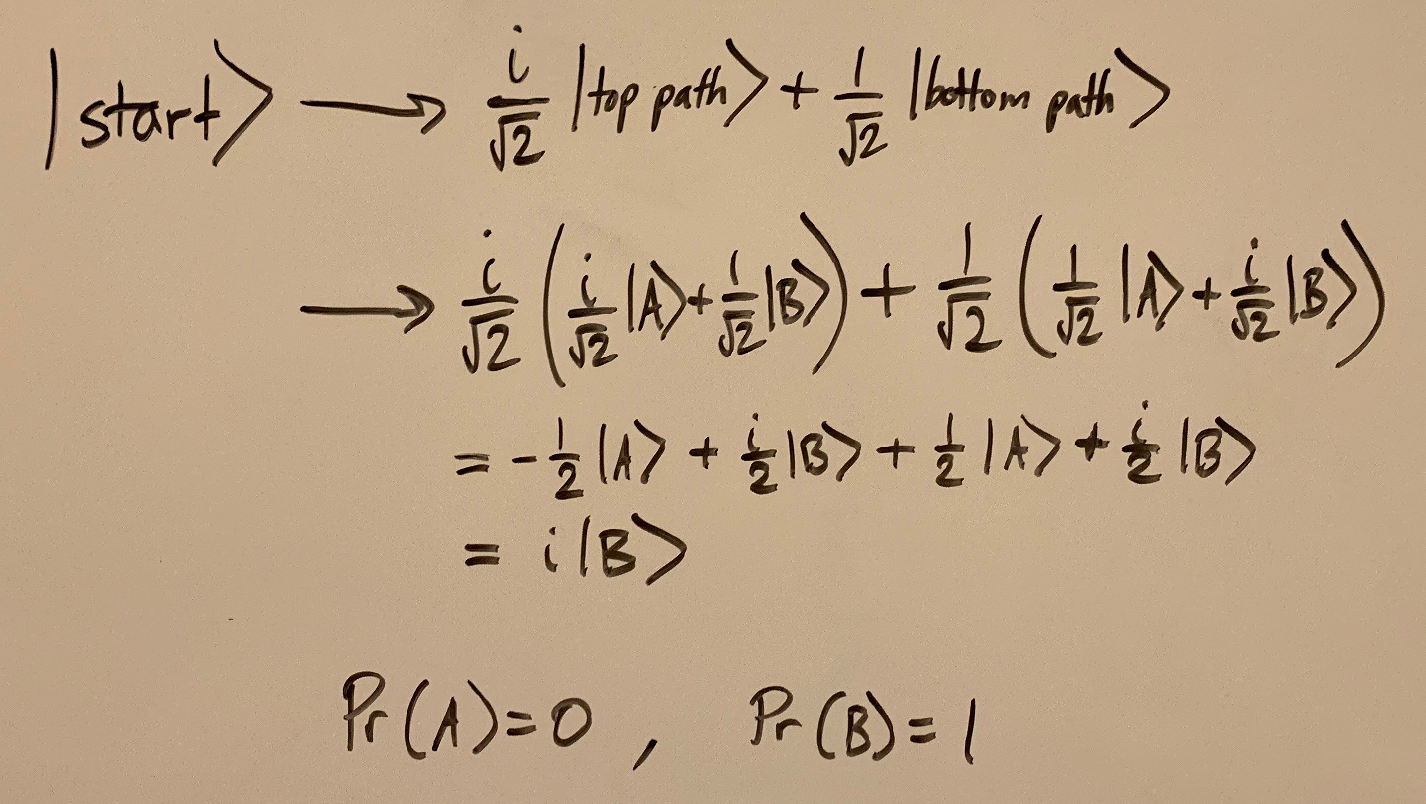
But it’s also just as wrong to say that the particle is in either one state or the other. Again, particles simply do not behave this way. Throw a bunch of electrons, one at a time, through a pair of thin slits in a wall and see how they spread out when they hit a screen on the other side. What you’ll get is a pattern that is totally inconsistent with the image of the electrons always being either at one location or the other. Instead, the pattern you’d get only makes sense under the assumption that the particle traveled through both slits and then interfered with itself.

If a superposition of A and B is not the same as “A and B’ and it’s not the same as ‘A or B’, then what is it? Well, it’s just that: a superposition! A superposition is something fundamentally new, with some of the features of “and” and some of the features of “or”. We can do no better than to describe the empirically observed features and then give that cluster of features a name.

Now, quantum mechanics tells us that for any two possible states that a system can be in, there is another state that corresponds to the system being in a superposition of the two. In fact, there’s an infinity of such superpositions, each corresponding to a different weighting of the two states.
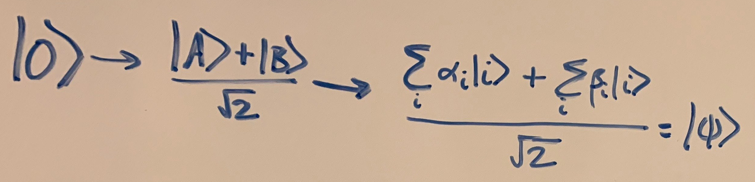
The Schrödinger equation is what tells how quantum mechanical systems evolve over time. And since all of nature is just one really big quantum mechanical system, the Schrödinger equation should also tell us how we evolve over time. So what does the Schrödinger equation tell us happens when we take a particle in a superposition of A and B and make a measurement of it?

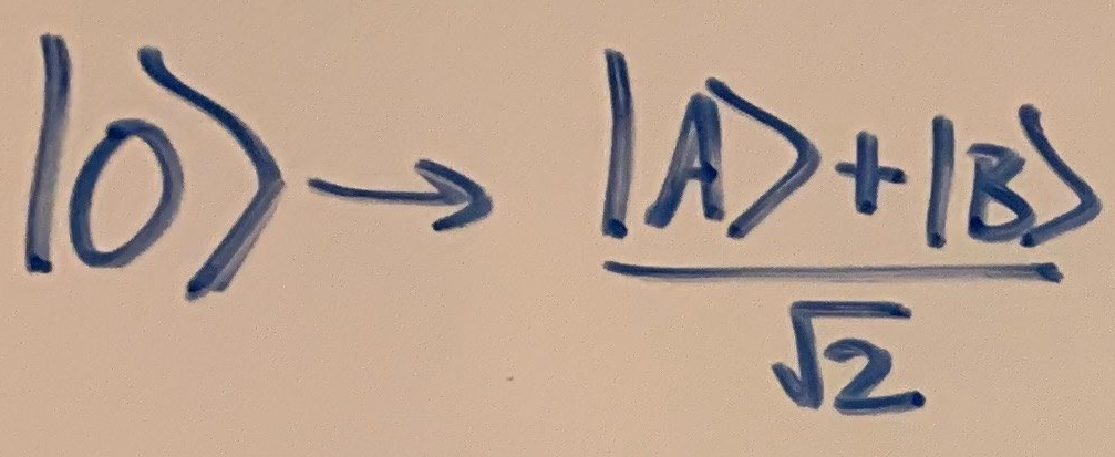
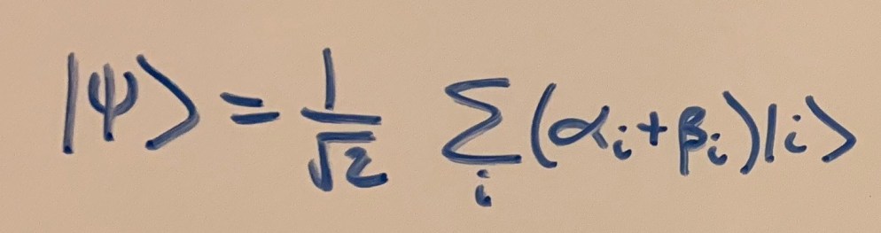
The answer is clear and unambiguous: The Schrödinger equation tells us that we ourselves enter into a superposition of states, one in which we observe the particle in state A, the other in which we observe it in B. This is a pretty bizarre and radical answer! The first response you might have may be something like “When I observe things, it certainly doesn’t seem like I’m entering into a superposition… I just look at the particle and see it in one state or the other. I never see it in this weird in-between state!”

But this is not a good argument against the conclusion, as it’s exactly what you’d expect by just applying the Schrödinger equation! When you enter into a superposition of “observing A” and “observing B”, neither branch of the superposition observes both A and B. And naturally, since neither branch of the superposition “feels” the other branch, nobody freaks out about being superposed.

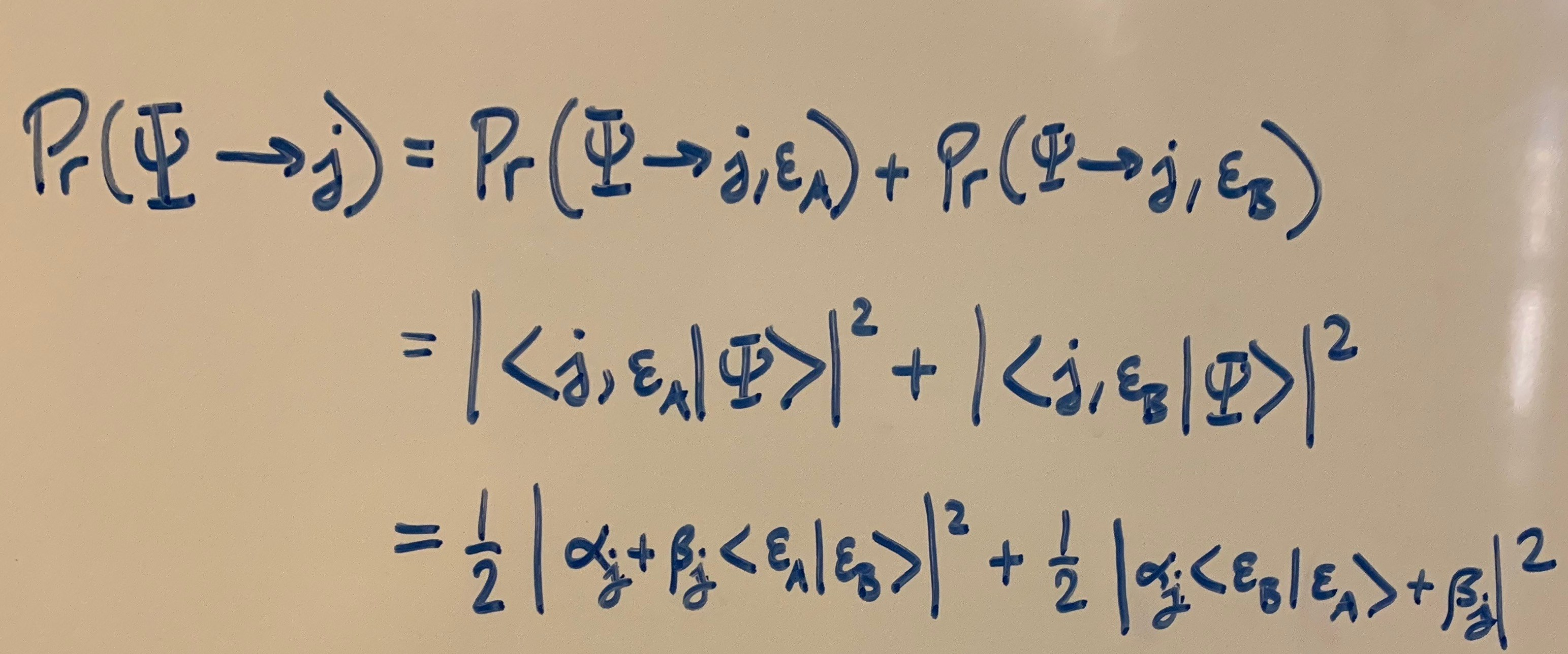
But there is a problem here, and it’s a serious one. The problem is the following: Sure, it’s compatible with our experience to say that we enter into superpositions when we make observations. But what predictions does it make? How do we take what the Schrödinger equation says happens to the state of the world and turn it into a falsifiable experimental setup? The answer appears to be that we can’t. At least, not using just the Schrödinger equation on its own. To get out predictions, we need an additional postulate, known as the Born rule.

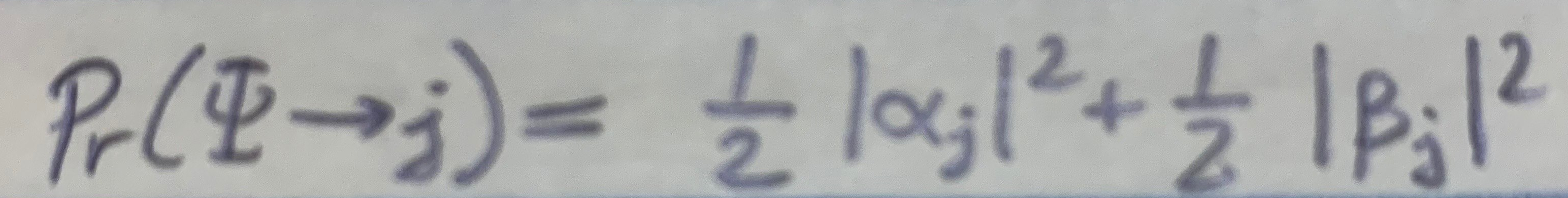
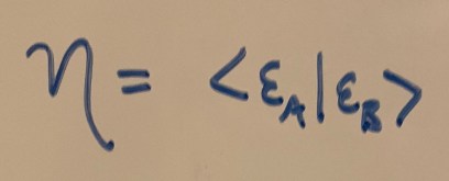
This postulate says the following: For a system in a superposition, each branch of the superposition has an associated complex number called the amplitude. The probability of observing any particular branch of the superposition upon measurement is simply the square of that branch’s amplitude.

For example: A particle is in a superposition of positions A and B. The amplitude attached to A is 0.8. The amplitude attached to B is 0.4. If we now observe the position of the particle, we will find it to be at either A with probability (.6)2 (i.e. 36%), or B with probability (.8)2 (i.e. 64%).

Simple enough, right? The problem is to figure out where the Born rule comes from and what it even means. The rule appears to be completely necessary to make quantum mechanics a testable theory at all, but it can’t be derived from the Schrödinger equation. And it’s not at all inevitable; it could easily have been that probabilities associated with the amplitude were gotten by taking absolute values rather than squares. Or why not the fourth power of the amplitude? There’s a substantive claim here, that probabilities associate with the square of the amplitudes that go into the Schrödinger equation, that needs to be made sense of. There are a lot of different ways that people have tried to do this, and I’ll list a few of the more prominent ones here.

The Copenhagen Interpretation

(Prepare to be disappointed.) The Copenhagen interpretation, which has historically been the dominant position among working physicists, is that the Born rule is just an additional rule governing the dynamics of quantum mechanical systems. Sometimes systems evolve according to the Schrödinger equation, and sometimes according to the Born rule. When they evolve according to the Schrödinger equation, they split into superpositions endlessly. When they evolve according to the Born rule, they collapse into a single determinate state. What determines when the systems evolve one way or the other? Something measurement something something observation something. There’s no real consensus here, nor even a clear set of well-defined candidate theories.

If you’re familiar with the way that physics works, this idea should send your head spinning. The claim here is that the universe operates according to two fundamentally different laws, and that the dividing line between the two hinges crucially on what we mean by the words “measurement and “observation. Suffice it to say, if this was the right way to understand quantum mechanics, it would go entirely against the spirit of the goal of finding a fundamental theory of physics. In a fundamental theory of physics, macroscopic phenomena like measurements and observations need to be built out of the behavior of lots of tiny things like electrons and quarks, not the other way around. We shouldn’t find ourselves in the position of trying to give a precise definition to these words, debating whether frogs have the capacity to collapse superpositions or if that requires a higher “measuring capacity”, in order to make predictions about the world (as proponents of the Copenhagen interpretation have in fact done!).

The Copenhagen interpretation is not an elegant theory, it’s not a clearly defined theory, and it’s fundamentally at tension with the project of theoretical physics. So why has it been, as I said, the dominant approach over the last century to understanding quantum mechanics? This really comes down to physicists not caring enough about the philosophy behind the physics to notice that the approach they are using is fundamentally flawed. In practice, the Copenhagen interpretation works. It allows somebody working in the lab to quickly assess the results of their experiments and to make predictions about how future experiments will turn out. It gives the right empirical probabilities and is easy to implement, even if the fuzziness in the details can start to make your head hurt if you start to think about it too much. As Jean Bricmont said, “You can’t blame most physicists for following this ‘shut up and calculate’ ethos because it has led to tremendous develop­ments in nuclear physics, atomic physics, solid­ state physics and particle physics.” But the Copenhagen interpretation is not good enough for us. A serious attempt to make sense of quantum mechanics requires something more substantive. So let’s move on.

Objective Collapse Theories

These approaches hinge on the notion that the Schrödinger equation really is the only law at work in the universe, it’s just that we have that equation slightly wrong. Objective collapse theories add slight nonlinearities to the Schrödinger equation so that systems sometimes spread out in superpositions and other times collapse into definite states, all according to one single equation. The most famous of these is the spontaneous collapse theory, according to which quantum systems collapse with a probability that grows with the number of particles in the system.

This approach is nice for several reasons. For one, it gives us the Born rule without requiring a new equation. It makes sense of the Born rule as a fundamental feature of physical reality, and makes precise and empirically testable predictions that can distinguish it from from other interpretations. The drawback? It makes the Schrödinger equation ugly and complicated, and it adds extra parameters that determine how often collapse happens. And as we know, whenever you start adding parameters you run the risk of overfitting your data.

Hidden Variable Theories

These approaches claim that superpositions don’t really exist, they’re just a high-level consequence of the unusual behavior of the stuff at the smallest level of reality.  They deny that the Schrödinger equation is truly fundamental, and say instead that it is a higher-level approximation of an underlying deterministic reality. “Deterministic?! But hasn’t quantum mechanics been shown conclusively to be indeterministic??” Well, not entirely. For a while there was a common sentiment amongst physicists that John Von Neumann and others had proved beyond a doubt that no deterministic theory could make the predictions that quantum mechanics makes. Later subtle mistakes were found in these purported proofs that left a door open for determinism. Today there are well-known fleshed-out hidden variable theories that successfully reproduce the predictions of quantum mechanics, and do so fully deterministically.

The most famous of these is certainly Bohmian mechanics, also called pilot wave theory. Here’s a nice video on it if you’d like to know more, complete with pretty animations. Bohmian mechanics is interesting, appear to work, give us the Born rule, and is probably empirically distinguishable from other theories (at least in principle). A serious issue with it is that it requires nonlocality, which is a challenge to any attempt to make it consistent with special relativity. Locality is such an important and well-understood feature of our reality that this constitutes a major challenge to the approach.

Many-Worlds / Everettian Interpretations

Ok, finally we talk about the approach that is most interesting in my opinion, and get to the title of this post. The Many-Worlds interpretation says, in essence, that we were wrong to ever want more than the Schrödinger equation. This is the only law that governs reality, and it gives us everything we need. Many-Worlders deny that superpositions ever collapse. The result of us performing a measurement on a system in superposition is simply that we end up in superposition, and that’s the whole story!

So superpositions never collapse, they just go deeper into superposition. There’s not just one you, there’s every you, spread across the different branches of the wave function of the universe. All these yous exist beside each other, living out all your possible life histories.

But then where does Many-Worlds get the Born rule from? Well, uh, it’s kind of a mystery. The Born rule isn’t an additional law of physics, because the Schrödinger equation is supposed to be the whole story. It’s not an a priori rule of rationality, because as we said before probabilities could have easily gone as the fourth power of amplitudes, or something else entirely. But if it’s not an a posteriori fact about physics, and also not an a priori knowable principle of rationality, then what is it?

This issue has seemed to me to be more and more important and challenging for Many-Worlds the more I have thought about it. It’s hard to see what exactly the rule is even saying in this interpretation. Say I’m about to make a measurement of a system in a superposition of states A and B. Suppose that I know the amplitude of A is much smaller than the amplitude of B. I need some way to say “I have a strong expectation that I will observe B, but there’s a small chance that I’ll see A.” But according to Many-Worlds, a moment from now both observations will be made. There will be a branch of the superposition in which I observe A, and another branch in which I observe B. So what I appear to need to say is something like “I am much more likely to be the me in the branch that observes B than the me that observes A.” But this is a really strange claim that leads us straight into the thorny philosophical issue of personal identity.

In what sense are we allowed to say that one and only one of the two resulting humans is really going to be you? Don’t both of them have equal claim to being you? They each have your exact memories and life history so far, the only difference is that one observed A and the other B. Maybe we can use anthropic reasoning here? If I enter into a superposition of observing-A and observing-B, then there are now two “me”s, in some sense. But that gives the wrong prediction! Using the self-sampling assumption, we’d just say “Okay, two yous, so there’s a 50% chance of being each one” and be done with it. But obviously not all binary quantum measurements we make have a 50% chance of turning out either way!

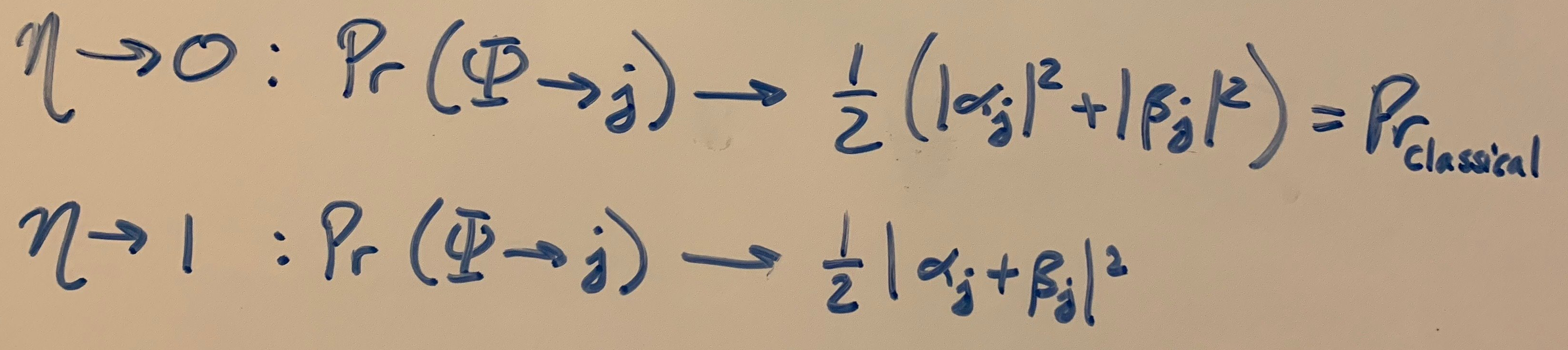
Maybe we can say that the world actually splits into some huge number of branches, maybe even infinite, and the fraction of the total branches in which we observe A is exactly the square of the amplitude of A? But this is not what the Schrödinger equation says! The Schrödinger equation tells exactly what happens after we make the observation: we enter a superposition of two states, no more, no less. We’re importing a whole lot into our interpretive apparatus by interpreting this result as claiming the literal existence of an infinity of separate worlds, most of which are identical, and the distribution of which is governed by the amplitudes.

What we’re seeing here is that Many-Worlds, by being too insistent on the reality of the superposition, the sole sovereignty of the Schrödinger equation, and the unreality of collapse, ends up running into a lot of problems in actually doing what a good theory of physics is supposed to do: making empirical predictions. The Many-Worlders can of course use the Born Rule freely to make predictions about the outcomes of experiments, but they have little to say in answer to what, in their eyes, this rule really amounts to. I don’t know of any good way out of this mess.

Basically where this leaves me is where I find myself with all of my favorite philosophical topics; totally puzzled and unsatisfied with all of the options that I can see.