The Cournot model is a simple economic model used to describe what happens when multiple companies compete with one another to produce some homogenous product. I’ve been playing with it a bit and ended up solving the general linear case. I assume that this solution is already known by somebody, but couldn’t find it anywhere. So I will post it here! It gives some interesting insight into the way that less-than-perfectly-competitive markets operate. First let’s talk about the general structure of the Cournot model.
Suppose we have n firms. Each produces some quantity of the product, which we’ll label as 
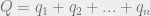


For each firm, there is some cost to producing the good. We capture this by giving each firm a cost function 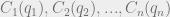


If we now assume that all firms are maximizing profit, we can find the outputs of each firm by taking the derivative of the profit and setting it to zero. 
Of course, without any more assumptions about the functions 

In the linear Cournot model, we write that 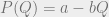


The constants 
Now we can write out the profit-maximization equations for the linear Cournot model. 


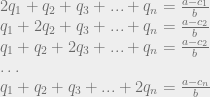
Translating this to a matrix equation…

Now if we could only find the inverse of the first matrix, we’d have our solution!

I found the inverse of this matrix by using the symmetry in the matrix to decompose it into two matrices that were each easier to work with:
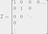
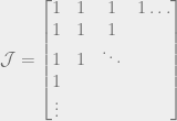

As a hypothesis, suppose that the inverse matrix has a similar form (one value for the diagonal elements, and another value for all off-diagonal elements). This allows us to write an equation for the inverse matrix:

To solve this, we’ll use the following easily proven identities.

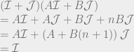


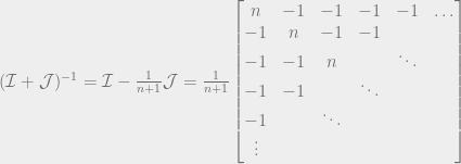
Alright awesome! Our hypothesis turned out to be true! (And it would have even if the entries in our matrix hadn’t been 1s and 2s. This is a really cool general method to find inverses of this family of matrices.) Now we just use this inverse matrix to solve for the output from each firm!
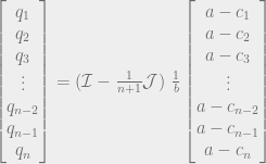
Define:

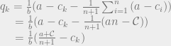
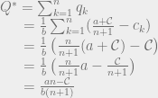
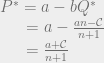

And there we have it, the full solution to the general linear Cournot model! Let’s discuss some implications of these results. First of all, let’s look at the two extreme cases: monopoly and perfect competition.
Monopoly: n = 1

Perfect Competition: n → ∞

The first observation is that the behavior of the market under monopoly looks very different from the case of perfect competition. For one thing, notice that the price under perfect competition is always going to be lower than the price under monopoly. This is a nice demonstration of the so-called monopoly markup. The quantity 

The flip side of the monopoly markup is that less of the good is produced and sold under a monopoly than under perfect competition. There are trades that could be happening (trades which would be mutually beneficial!) which do not occur. Think about it: the monopoly price is halfway between the cost of production and the highest bidder’s price. This means that there are a bunch of people that would buy the product at above the cost of production but below the monopoly price. And since the price they would buy it for is above the cost of production, this would be a profitable exchange for both sides! But alas, the monopoly doesn’t allow these trades to occur, as it would involve lowering the price for everybody, including those who are willing to pay a higher price, and thus decreasing net profit.
Things change as soon as another firm joins the market. This firm can profitably sell the good at a lower price than the monopoly price and snatch up all of their business. This introduces a downward pressure on the price. Here’s the exact solution for the case of duopoly.
Duopoly: n = 2

Interestingly, in the duopoly case the market price still rests at a value above the marginal cost of production for either firm. As more and more firms enter the market, competition pushes the price down further and further until, in the limit of perfect competition, it converges to the cost of production.
The implication of this is that in the limit of perfect competition, firms do not make any profit! This may sound a little unintuitive, but it’s the inevitable consequence of the line of argument above. If a bunch of companies were all making some profit, then their price is somewhere above the cost of production. But this means that one company could slightly lower its price, thus snatching up all the customers and making massively more money than its competitors. So its competitors will all follow suit, pushing down their prices to get back their customers. And in the end, all the firms will have just decreased their prices and their profits, even though every step in the sequence appeared to be the rational and profitable action by each firm! This is just an example of a coordination problem. If the companies could all just agree to hold their price fixed at, say, the monopoly price, then they’d all be better off. But each individual has a strong monetary incentive to lower their price and gather all the customers. So the price will drop and drop until it can drop no more (that is, until it has reached the cost of production, at which point it is no longer profitable for a company to lower their price).
This implies that in some sense, the limit of perfect competition is the best possible outcome for consumers and the worst outcome for producers. Every consumer that values the product above the cost of its production will get it, and they will all get it at the lowest possible price. So the consumer surplus will be enormous. And companies producing the product make no net profit; any attempt to do so immediately loses them their entire customer base. (In which case, what is the motivation for the companies to produce the product in the first place? This is known as the Bertrand paradox.)
We can also get the easier-to-solve special case where all firms have the same cost of production.
Equal Production Costs


It’s curious that in the Cournot model, prices don’t immediately drop to production levels as soon you go from a monopoly to a duopoly. After all, the intuitive argument I presented before works for two firms: if both firms are pricing the goods at any value above zero, then each stands to gain by lowering the price a slight bit and getting all the customers. And this continues until the price settles at the cost of production. We didn’t build in any ability of the firms to collude to the model, so what gives? What the Cournot model tells us is certainly more realistic (we don’t expect a duopoly to behave like a perfectly competitive market), but where does this realism come from?
The answer is that in a certain sense we did build in collusion between firms from the start, in the form of agreement on what price to sell at. Notice that our model did not allow different firms to set different prices. In this model, firms compete only on quantity of goods sold, not prices. The price is set automatically by the consumer demand function, and no single individual can unilaterally change their price. This constraint is what gives us the more realistic-in-character results that we see, and also what invalidates the intuitive argument I’ve made here.
One final observation. Consider the following procedure. You line up a representative from each of the n firms, as well as the highest bidder for the product (representing the highest price at which the product could be sold). Each of the firms states their cost of production (the lowest they could profitably bring the price to), and the highest bidder states the amount that he values the product (the highest price at which he would still buy it). Now all of the stated costs are averaged, and the result is set as the market price of the good. Turns out that this procedure gives exactly the market price that the linear Cournot model predicts! This might be meaningful or just a curious coincidence. But it’s quite surprising to me that the slope of the demand curve (
Nicely done! This is a very clear explanation. One thing to be careful about is that there is an implicit constraint in the firms’ optimization problem which is that the quantity they choose to produce needs to be non-negative.
Thanks!! Yes, that’s a good point. I thought a little bit about how to incorporate that constraint in while still analytically solving for q_k, but couldn’t come up with anything. Do you have any ideas as to how to do that?
Often times for optimization problems with inequality constraints, including this case, you can use the Kuhn-Tucker conditions to find necessary or possibly even sufficient conditions for the optimal solution. But for this case I don’t know how to make the math nice when there’s a large number of heterogeneous firms.