In the last post, we described what qubits are and how quantum computing involves the manipulation of these qubits to perform useful calculations.
In this post, we’ll abstract away from the details of the physics of qubits and just call the two observable states |0⟩ and |1⟩, rather than |ON⟩ and |OFF⟩. This will be useful for ultimately describing quantum algorithms. But before we get there, we need to take a few more steps into the details of quantum gates.
Recap: the general description of a qubit is |Ψ⟩ = α|0⟩ + β|1⟩, where α and β are called amplitudes, and |α|² and |β|² are the probabilities of observing the system in the state |0⟩ and |1⟩, respectively.
We can also express the states of qubits as vectors, like so:

Quantum gates are transformations from quantum states to other quantum states. We can express these transformations as matrices, which when applied to state vectors yield new state vectors. Here’s a simple example of a quantum gate called the X gate:

Applied to the states |0⟩ and |1⟩, this gate yields

Applied to any general state, this gate yields:

Another gate that is used all the time is the Hadamard gate, or H gate.

Let’s see what it does to the |0⟩ and |1⟩ states:

In words, H puts ordinary states into superposition. Superposition is the key to quantum computing. Without it, all we have is a fancier way of talking about classical computing. So it should make sense that H is a very useful gate.
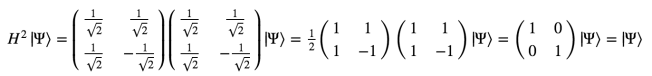
One more note on H: When you apply it to a state twice, you get back the state you started with. A simple proof of this comes by just multiplying the H matrix by itself:
Okay, enough with single qubits. While they’re pretty cool as far as they go, any non-trivial quantum algorithm is going to involve multiple qubits.
It turns out that everything we’ve said so far generalizes quite nicely. If we have two qubits, we describe the combined system by smushing them together with what’s called a tensor product (denoted ⊗). What this ends up looking like is the following:

The first number refers to the state of the first qubit, and the second refers to the state of the second.
Let’s smush together two arbitrary qubits:

This is pretty much exactly what we should have expected combining qubit states would look like.
The amplitude for the combined state to be |00⟩ is just the product of the amplitude for the first qubit to be |0⟩ and the second to be |0⟩. The amplitude for the combined state to be |01⟩ is just the product of the amplitude for the first qubit to be |0⟩ and second to be |1⟩. And so on.
We can write a general two qubit state as a vector with four components.

And as you might expect by now, two-qubit gates are simply 4 by 4 matrices that act on such vectors to produce new vectors. For instance, we can calculate the 4×4 matrix corresponding to the action of a Hadamard gate on both qubits:
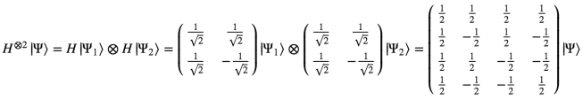
Why the two-qubit Hadamard gate has this exact form is a little beyond the scope of this post. Suffice it to say that this is the 4×4 matrix that successfully transforms two qubits as if they had each been put through a single-qubit Hadamard gate. (You can verify this for yourself by simply applying H to each qubit individually and then smushing them together in the way we described above.)
Here’s what the two-qubit Hadamard gate does to the four basic two-qubit states.

Here’s a visual representation of this transformation using bar graphs:

We can easily extend this further to three, four, or more qubits. The state vector describing a N-qubit system must consider the amplitude for all possible combinations of 0s and 1s for each qubit. There are 2ᴺ such combinations (starting at 00…0 and ending at 11…1). So the vector describing an N-qubit system is composed of 2ᴺ complex numbers.
If you’ve followed everything so far, then we are now ready to move on to some actual quantum algorithms! In the next post, we’ll see first how qubits can be used to solve problems that classical bits cannot, and then why quantum computers have this enhanced problem-solving ability.

6 thoughts on “More on quantum gates”