(Note: in here are spoilers for my puzzle a couple days ago. Also, familiarity with both lambda calculus and lambda diagrams is assumed; here’s a link for the latter.)
In lambda calculus, numbers are sort of like adverbs; they tell you how many times to do something. So “2” is like “twice”; it’s a function that takes in an f and an x and returns f of f of x, written in lambda calculus as f (f x). “3” is like “thrice”; 3 f x = f (f (f x)).
One of the reasons that this turns out to be a really nice definition of numbers is that it makes arithmetic very simple, especially with large numbers. For instance, the operation of taking a number to the power of another number can be defined extremely simply as follows:
↑ = λnm.m n
In other words, we do an m-fold application of the operation “do an n-fold application.”
Once we’ve defined exponentiation, we can pretty easily get tetration too. n ↑↑ m is defined to be n ↑ (n ↑ (… ↑ n)), with m copies of n. But this is just m-fold application of the operation (n ↑) to 1. So we can write:
↑↑ = λnm.m (↑ n) 1
Similarly, for pentation (or hyper-5), we can write:
↑↑↑ = λnm.m (↑↑ n) 1
And in general, for any n, we can write:
↑N+1 = λnm.m (↑N n) 1
Together with our definition of ↑, this gives us a nice construction of all the hyperoperations:
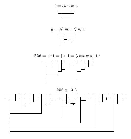
↑ = λnm.m n
↑N+1 = λnm.m (↑N n) 1
There’s a problem though. If we actually tried to write out something like ↑100 just in terms of the basic syntax of the lambda calculus, our expression would end up extremely long; we’d have to write something like ↑99, ↑98, ↑97, and so on. We can do better than this by “automating” the process of going from ↑N to ↑N+1 (after all, we’re doing the same thing each time!). So we define a function that implements this process, arbitrarily choosing to name it g:
g = λfnm.m (f n) 1
Some examples of how g behaves:
↑↑= g ↑
↑↑↑ = g (↑↑) = g (g ↑)
↑↑↑↑ = g (↑↑↑) = g (g (g ↑))
You might already see where this is going. Now to get to ↑N+1, we just need to do an N-fold application of g to ↑! So we can write:
↑N+1 = N g ↑
Now writing out something massive like (3 ↑257 3) merely requires us writing out the functions g, ↑, 3, and 256, each of which is pretty simple. And the end result is much more concise than what we would have gotten using our previous construction.
There are the lambda diagrams for what we have so far:
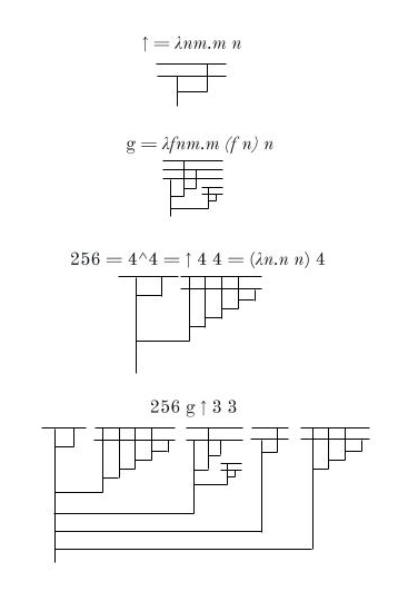
There’s a bit of redundancy here that can be removed, shrinking the diagrams:
But suppose now we want to go a step further. Let’s define the following extremely fast-growing sequence of numbers:
a0 = 1
a1 = 3 ↑(a0 + 1) 3
a2 = 3 ↑(a1 + 1) 3
…
Some of you may recognize this sequence as closely resembling the usual construction of Graham’s number. It’s not quite the same as this construction, but Graham’s number is approximately a66. This sequence can be encoded into lambda calculus using the same trick as before: define a new function which takes us from aN to aN+1, and then apply it n-fold to a0. Let’s call this function h.
h = λa.a g ↑ 3 3
Verify for yourself that h takes us from one number in our sequence to the next!
a1 = h a0
a2 = h a1 = h (h a0) = 2 h a0
a3 = h a2 = h (h a1) = h (h (h a0)) = 3 h a0
We can construct a general function now that takes in a number n and returns an:
a = λn.n h a0
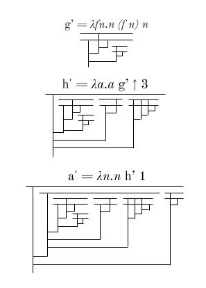
We can do a little better than this by removing some redundancy. Notice the repeated 3s in the definition of h; we can built this repetition into our definition of g and get an even more concise representation of massive numbers.
g’ = λfn.n (f n) n
h’ = λa.a g ↑ 3
a’ = λn.n h’ 1
Here’s what these new and improved functions look like:
And finally, here’s an image of a256, much much larger than Graham’s number, to hang on your wall:
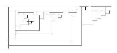
Keep in mind that Graham’s number is really really big. From wiki: “it is so large that the observable universe is far too small to contain an ordinary digital representation of Graham’s number, assuming that each digit occupies one Planck volume, possibly the smallest measurable space. But even the number of digits in this digital representation of Graham’s number would itself be a number so large that its digital representation cannot be represented in the observable universe. Nor even can the number of digits of that number—and so forth, for a number of times far exceeding the total number of Planck volumes in the observable universe.”
It’s pretty wild to think that if you start applying beta reductions to this diagram, the lambda diagram you’ll build up (the normal form of the expression) will be so large that it could not be represented within the entire observable universe!
