This is part 4 of my series on quantum computing. The earlier posts provide necessary background material.
Part 1: Quantum Computing in a Nutshell
Part 2: More on quantum gates
Part 3: Deutch-Josza Algorithm

Grover’s algorithm

This algorithm involves searching through an unsorted list for a particular item. Let’s first look at how this can be optimally solved classically.

Suppose you have private access to the following list:

1. apple
2. banana
3. grapefruit
4. kiwi
5. guava
6. mango
7. lemon
8. papaya

A friend of yours wants to know where on the list they could find guava. They are allowed to ask you questions like “Is the first item on the list guava?” and “Is the nth item on the list gauva?”, for any n they choose. Importantly, they have no information about the ordering of your list.

How many queries do they need to perform in order to answer this question?

Well, since they have no information about its placement, they can do no better than querying random items in the list and checking them off one by one. In the best case, they find it on their first query. And in the worst case, they find it on their last query. Thus, if the list is of length N, the number of queries in the average case is N/2.

Grover’s algorithm solves the same problem with roughly √N queries. This is only a quadratic speedup, but still should seem totally impossible. What this means is that in a list of 1,000,000 items, you can find any item of your choice with only about 1,000 queries.

Let’s see how.

Firstly, we can think about the search problem as a function-analysis problem. We’re not really interested in what the items in the list are, just whether or not the item is guava. So we can transform our list of items into a simple binary function: 0 if the input is not the index of the item ‘guava’ and 1 if the input is the index of the item ‘guava’. Now our list looks like:

Our challenge is now to find out for which value of x f(x) returns 1.

Now, this algorithm uses three quantum gates. Two of them we’ve already seen: H^⊗N and U_f. I’ll remind you what these two do:

The third is called the Grover diffusion operator, D. In words, what D does to a state Ψ is reflect it over the average amplitude in Ψ. Visually, this looks like:

Mathematically, this transformation can be defined as follows:

Check for yourself that 2ā – a_x flips the amplitude a_x over ā. We are guaranteed that D is a valid quantum gate because it keeps the state normalized (the average amplitude remains the same after the flip).

Now, with H^⊗N, U_f , and D in hand, we are ready to present the algorithm:

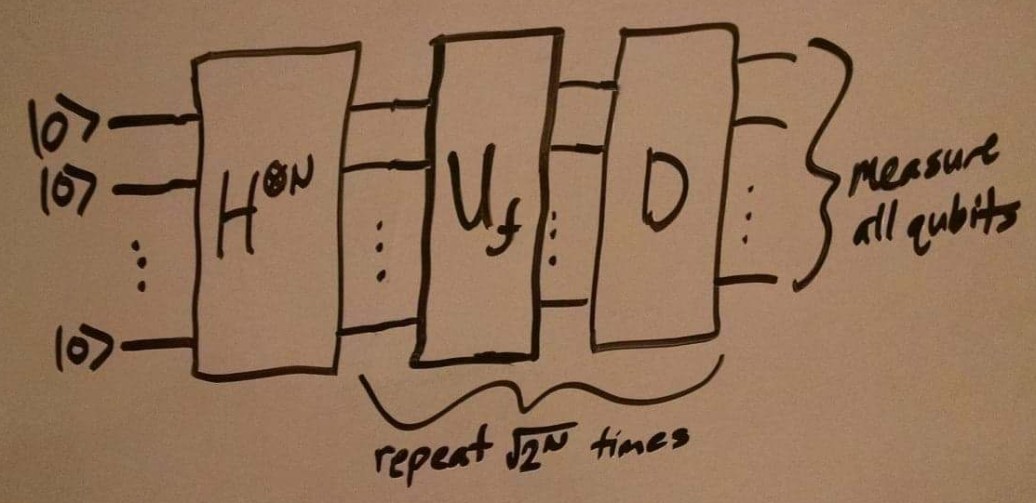
We start with all N qubits in the state |00…0⟩, and apply the Hadamard gate to put them in a uniform superposition. Then we apply U_f  to flip the amplitude of the desired input, and D to flip the whole superposition over the average. We repeat this step square root of the length of the list times, and then measure the qubits.

Here’s a visual intuition for why this works. Let’s suppose that N=3 (so our list contains 8 items), and the item we’re looking for is the 5th in the list (100 in binary). Here is each step in the algorithm:

You can see that what the combination of U_f  and D does to the state is that it magnifies the amplitude of the desired value of f. As you do this again and again, the amplitude is repeatedly magnified, reaching a maximum after sqrt(2^N) repeats.

And that’s Grover’s algorithm! Once again we see that the key to it is the unusual phenomenon of superposition. By putting the state into superposition in our first step, we manage to make each individual query give us information about all possible inputs. And through a little cleverness, we are able to massage the amplitudes of our qubits in order that our desired output becomes overwhelmingly likely.

A difference between Grover’s algorithm and the Deutsch-Josza algorithm is that Grover’s algorithm is non-deterministic. It isn’t guaranteed with 100% probability of giving the right answer. But each run of the algorithm only delivers an incorrect answer with probability 1/2^N, which is an exponentially small error. Repeating the algorithm n times gives you the wrong answer with only (1/2^N)ⁿ probability. And so on.

While it is a more technically complicated algorithm than the Deutsch-Josza algorithm, I find Grover’s algorithm easier to intuitively understand. Let me know in the comments if anything remains unclear!

Next: Building the quantum oracle