Integrated information theory relates consciousness to degrees of integrated information within a physical system. I recently became interested in IIT and found it surprisingly hard to locate a good simple explanation of the actual mathematics of integrated information online.
Having eventually just read through all of the original papers introducing IIT, I discovered that integrated information is closely related to some of my favorite bits of mathematics, involving information theory and causal modeling. This was exciting enough to me that I decided to write a guide to understanding integrated information. My goal in this post is to introduce a beginner to integrated information in a rigorous and (hopefully!) intuitive way.
I’ll describe it increasing levels of complexity, so that even if you eventually get lost somewhere in the post, you’ll be able to walk away having learned something. If you get to the end of this post, you should be able to sit down with a pencil and paper and calculate the amount of integrated information in simple systems, as well as how to calculate it in principle for any system.
Level 1
So first, integrated information is a measure of the degree to which the components of a system are working together to produce outputs.
A system composed of many individual parts that are not interacting with each other in any way is completely un-integrated – it has an integrated information ɸ = 0. On the other hand, a system composed entirely of parts that are tightly entangled with one another will have a high amount of integrated information, ɸ >> 0.
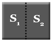
For example, consider a simple model of a camera sensor.

This sensor is composed of many independent parts functioning completely separately. Each pixel stores a unit of information about the outside world, regardless of what its neighboring pixels are doing. If we were to somehow sever the causal connections between the two halves of the sensor, each half would still capture and store information in exactly the same way.
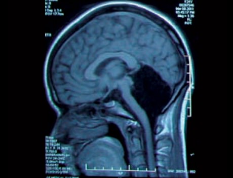
Now compare this to a human brain.

The nervous system is a highly entangled mesh of neurons, each interacting with many many neighbors in functionally important ways. If we tried to cut the brain in half, severing all the causal connections between the two sides, we would get an enormous change in brain functioning.
Makes sense? Okay, on to level 2.
Level 2
So, integrated information has to do with the degree to which the components of a system are working together to produce outputs. Let’s delve a little deeper.
We just said that we can tell that the brain is integrating lots of information, because the functioning would be drastically disrupted if you cut it in half. A keen reader might have realized that the degree to which the functioning is disrupted will depend a lot on how you cut it in half.
For instance, cut off the front half of somebody’s brain, and you will end up with total dysfunction. But you can entirely remove somebody’s cerebellum (~50% of the brain’s neurons), and end up with a person that has difficulty with coordination and is a slow learner, but is otherwise a pretty ordinary person.
What this is really telling us is that different parts of the brain are integrating information differently. So how do we quantify the total integration of information of the brain? Which cut do we choose when evaluating the decrease in functioning?
Simple: We look at every possible way of partitioning the brain into two parts. For each one, we see how much the brain’s functioning is affected. Then we locate the minimum information partition, that is, the partition that results in the smallest change in brain functioning. The change in functioning that results from this particular partition is the integrated information!
Okay. Now, what exactly do we mean by “changes to the system’s functioning”? How do we measure this?
Answer: The functionality of a system is defined by the way in which the current state of the system constrains the past and future states of the system.
To make full technical sense of this, we have to dive a little deeper.
Level 3
How many possible states are there of a Connect Four board?
(I promise this is relevant)
The board is 6 by 7, and each spot can be either a red piece, a black piece, or empty.

So a simple upper bound on the number of total possible board states is 342 (of course, the actual number of possible states will be much lower than this, since some positions are impossible to get into).
Now, consider what you know about the possible past and future states of the board if the board state is currently…

Clearly there’s only one possible past state:
And there are seven possible future states:


What this tells us is that the information about the current state of the board constrains the possible past and future states, selecting exactly one possible board out of the 342 possibilities for the past, and seven out of 342 possibilities for the future.
More generally, for any given system S we have a probability distribution over past and future states, given that the current state is X.

Pfuture(X, S) = Pr( Future state of S | Present state of S is X )
Ppast(X, S) = Pr( Past state of S | Present state of S is X )
For any partition of the system into two components, S1 and S2, we can consider the future and past distributions given that the states of the components are, respectively, X1 and X2, where X = (X1, X2).
Pfuture(X, S1, S2) = Pr( Future state of S1 | Present state of S1 is X1 )・Pr( Future state of S2 | Present state of S2 is X2 )
Ppast(X, S1, S2) = Pr( Past state of S1 | Present state of S1 is X1 )・Pr( Past state of S2 | Present state of S2 is X2 )
Now, we just need to compare our distributions before the partition to our distributions after the partition. For this we need some type of distance function D that assesses how far apart two probability distributions are. Then we define the cause information and the effect information for the partition (S1, S2).
Cause information = D( Ppast(X, S), Ppast(X, S1, S2) )
Effect information = D( Pfuture(X, S), Pfuture(X, S1, S2) )
In short, the cause information is how much the distribution over past states changes when you partition off your system into two separate systems And the future information is the change in the distribution over future states when you partition the system.
The cause-effect information CEI is then defined as the minimum of the cause information CI and effect information EI.
CEI = min{ CI, EI }
We’ve almost made it all the way to our full definition of ɸ! Our last step is to calculate the CEI for every possible partition of S into two pieces, and then select the partition that minimizes CEI (the minimum information partition MIP).
The integrated information is just the cause effect information of the minimum information partition!
ɸ = CEI(MIP)
Level 4
We’ve now semi-rigorously defined ɸ. But to really get a sense of how to calculate ɸ, we need to delve into causal diagrams. At this point, I’m going to assume familiarity with causal modeling. The basics are covered in a series of posts I wrote starting here.
Here’s a simple example system:

This diagram tells us that the system is composed of two variables, A and B. Each of these variables can take on the values 0 and 1. The system follows the following simple update rule:
A(t + 1) = A(t) XOR B(t)
B(t + 1) = A(t) AND B(t)
We can redraw this as a causal diagram from A and B at time 0 to A and B at time 1:

What this amounts to is the following system evolution rule:
ABt → ABt+1
00 00
01 10
10 10
11 01
Now, suppose that we know that the system is currently in the state AB = 00. What does this tell us about the future and past states of the system?
Well, since the system evolution is deterministic, we can say with certainty that the next state of the system will be 00. And since there’s only one way to end up in the state 00, we know that the past state of the system 00.
We can plot the probability distributions over the past and future distributions as follows:

This is not too interesting a distribution… no information is lost or gained going into the past or future. Now we partition the system:

The causal diagram, when cut, looks like:
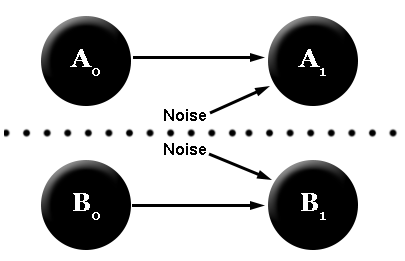
Why do we have the two “noise” variables? Well, both A and B take two variables as inputs. Since one of these causal inputs has been cut off, we replace it with a random variable that’s equally likely to be a 0 or a 1. This procedure is called “noising” the causal connections across the partition.
According to this diagram, we now have two independent distributions over the two parts of the system, A and B. In addition, to know the total future state of a system, we do the following:
P(A1, B1 | A0, B0) = P(A1 | A0) P(B1 | B0)
We can compute the two distributions P(A1 | A0) and P(B1 | B0) straightforwardly, by looking at how each variable evolves in our new causal diagram.
A0 = 0 ⇒ A1 = 0, 1 (½ probability each)
B0 = 0 ⇒ B1 = 0
A0 = 0 ⇒ A-1 = 0, 1 (½ probability each)
B0 = 0 ⇒ B-1 = 0, 1 (probabilities ⅔ and ⅓)
This implies the following probability distribution for the partitioned system:

I recommend you go through and calculate this for yourself. Everything follows from the updating rules that define the system and the noise assumption.
Good! Now we have two distributions, one for the full system and one for the partitioned system. How do we measure the difference between these distributions?
There are a few possible measures we could use. My favorite of these is the Kullback-Leibler divergence DKL. Technically, this metric is only used in IIT 2.0, not IIT 3.0 (which uses the earth-mover’s distance). I prefer DKL, as it has a nice interpretation as the amount of information lost when the system is partitioned. I have a post describing DKL here.
Here’s the definition of DKL:
DKL(P, Q) = ∑ Pi log(Pi / Qi)
We can use this quantity to calculate the cause information and the effect information:
Cause information = log(3) ≈ 1.6
Effect information = log(2) = 1
These values tell us that our partition destroys about .6 more bits of information about the past than it does the future. For the purpose of integrated information, we only care about the smaller of these two (for reasons that I don’t find entirely convincing).
Cause-effect information = min{ 1, 1.6 } = 1
Now, we’ve calculated the cause-effect information for this particular partition. And since our system has only two variables, this is the only possible partition.
The integrated information is the cause-effect information of the minimum information partition. Since our system only has two components, the partition we’ve examined is the only possible partition, meaning that it must be the minimum information partition. And thus, we’ve calculated ɸ for our system!
ɸ = 1
Level 5
Let’s now define ɸ in full generality.
Our system S consists of a vector of N variables X = (X1, X2, X3, …, XN), each an element in some space 𝒳. Our system also has an updating rule, which is a function f: 𝒳N → 𝒳N. In our previous example, 𝒳 = {0, 1}, N = 2, and f(x, y) = (x XOR y, x AND y).
More generally, our updating rule f can map X to a probability distribution p: 𝒳N → ℝ. We’ll denote P(Xt+1 | Xt) as the distribution over the possible future states, given the current state. P is defined by our updating rule: P(Xt+1 | Xt) = f(Xt). The distribution over possible past states will be denoted P(Xt-1 | Xt). We’ll obtain this using Bayes’ rule: P(Xt-1 | Xt) = P(Xt | Xt-1) P(Xt-1) / P(Xt) = f(Xt-1) P(Xt-1) / P(Xt).
A partition of the system is a subset of {1, 2, 3, …, N}, which we’ll label A. We define B = {1, 2, 3, …, N} \ A. Now we can define XA = ( Xa )a∈A, and XB = ( Xb )b∈B. Loosely speaking, we can say that X = (XA, XB), i.e. that the total state is just the combination of the two partitions A and B.
We now define the distributions over future and past states in our partitioned system:
Q(Xt+1 | Xt) = P(XA, t+1 | XA, t) P(XB, t+1 | XB, t)
Q(Xt-1 | Xt) = P(XA, t-1 | XA, t) P(XB, t-1 | XB, t).
The effect information EI of the partition defined by A is the distance between P(Xt+1 | Xt) and Q(Xt+1 | Xt), and the cause information CI is defined similarly. The cause-effect information is defined as the minimum of these two.
CI(f, A, Xt) = D( P(Xt-1 | Xt), Q(Xt-1 | Xt) )
EI(f, A, Xt) = D( P(Xt+1 | Xt), Q(Xt+1 | Xt) )
CEI(f, A, Xt) = min{ CI(f, A, Xt), EI(f, A, Xt) }
And finally, we define the minimum information partition (MIP) and the integrated information:
MIP = argminA CEI(f, A, Xt)
ɸ(f, Xt) = minA CEI(f, A, Xt)
= CEI(f, MIP, Xt)
And we’re done!
Notice that our final result is a function of f (the updating function) as well as the current state of the system. What this means is that the integrated information of a system can change from moment to moment, even if the organization of the system remains the same.
By itself, this is not enough for the purposes of integrated information theory. Integrated information theory uses ɸ to define gradations of consciousness of systems, but the relationship between ɸ and consciousness isn’t exactly one-to-on (briefly, consciousness resides in non-overlapping local maxima of integrated information).
But this post is really meant to just be about integrated information, and the connections to the theory of consciousness are actually less interesting to me. So for now I’ll stop here! 🙂
