We can use the concepts in information theory that I’ve been discussing recently to discuss the idea of optimal experimental design. The main idea is that when deciding which experiment to run out of some set of possible experiments, you should choose the one that will generate the maximum information. Said another way, you want to choose experiments that are surprising as possible, since these provide the strongest evidence.
An example!
Suppose that you have a bunch of face-down cups in front of you. You know that there is a ping pong ball underneath one of the cups, and want to discover which one it is. You have some prior distribution of probabilities over the cups, and are allowed to check under exactly one cup. Which cup should you choose in order to get the highest expected information gain?
The answer to this question isn’t extremely intuitively obvious. You might think that you want to choose the cup that you think is most likely to hold the ball, because then you’ll be most likely to find the ball there and thus learn exactly where the ball is. But at the same time, the most likely choice of ball location is also the one that gives you the least information if the ball is actually there. If you were already fairly sure that the ball was under that cup, then you don’t learn much by discovering that it was.
Maybe instead the better strategy is to go for a cup that you think is fairly unlikely to be hiding the ball. Then you’ll have a small chance of finding the ball, but in that case will gain a huge amount of evidence. Or perhaps the maximum expected information gain is somewhere in the middle.
The best way to answer this question is to actually do the calculation. So let’s do it!
First, we’ll label the different theories about the cup containing the ball:
{C1, C2, C3, … CN}
Ck corresponds to the theory that the ball is under the kth cup. Next, we’ll label the possible observations you could make:
{X1, X2, X3, … XN}
Xk corresponds to the observation that the ball is under the kth cup.
Now, our prior over the cups will contain all of our past information about the ball and the cups. Perhaps we thought we heard a rattle when somebody bumped one of the cups earlier, or we notice that the person who put the ball under one of the cups was closer to the cups on the right hand side. All of this information will be contained in the distribution P:
(P1, P2, P3, … PN)
Pk is shorthand for P(Ck) – the probability of Ck being true.
Good! Now we are ready to calculate the expected information gain from any particular observation. Let’s say that we decide to observe X3. There are two scenarios: either we find the ball there, or we don’t.
Scenario 1: You find the ball under cup 3. In this case, you previously had a credence of P3 in X3 being true, so you gain -log(P3) bits of information.
Scenario 2: You don’t find the ball under cup 3. In this case, you gain –log(1 – P3) bits of information.
With probability P3, you gain –log(P3) bits of information, and with probability (1 – P3) you gain –log(1 – P3) bits of information. So your expected information gain is just –P3 logP3 – (1 – P3) logP3.
In general, we see that if you have a prior credence of P in the cup containing the ball, then your expected information gain is:
-P logP – (1 – P) logP
What does this function look like?
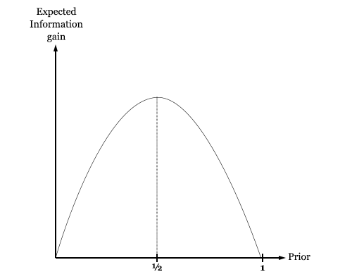
We see that it has a peak value at 50%. This means that you expect to gain the most information by looking at a cup that you are 50% sure contains the ball. If you are any more or less confident than this, then evidently you learn less than you would have if you were exactly agnostic about the cup.
Intuitively speaking, this means that we stand to learn the most by doing an experiment on a quantity that we are perfectly agnostic about. Practically speaking, however, the mandate that we run the experiment that maximizes information gain ends up telling us to always test the cup that we are most confident contains the ball. This is because if you split your credences among N cups, they will be mostly under 50%, so the closest you can get to 50% will be the largest credence.
Even if you are 99% confident that the fifteenth cup out of one hundred contains the ball, you will have just about .01% credence in each of the others containing the ball. Since 99% is closer to 50% than .01%, you will stand to gain the most information by testing the fifteenth ball (although you stand to gain very little information in a more absolute sense).
This generalizes nicely. Suppose that instead of trying to guess whether or not there is a ball under a cup, you are trying to guess whether there is a ball, a cube, or nothing. Now your expected information gain in testing a cup is a function of your prior over the cup containing a ball Pball, your prior over it containing a cube Pcube, and your prior over it containing nothing Pempty.
-Pball logPball – Pcube logPcube – Pempty logPempty
Subject to the constraint that these three priors must add up to 1, what set of (Pball, Pcube, Pempy) maximizes the information gain? It is just (⅓, ⅓, ⅓).
Optimal (Pball, Pcube, Pempy) = (⅓, ⅓, ⅓)
Imagine that you know that exactly one cup is empty, exactly one contains a cube, and exactly one contains a ball, and have the following distribution over the cups:
Cup 1: (⅓, ⅓, ⅓)
Cup 2: (⅔, ⅙, ⅙)
Cup 3: (0, ½, ½)
If you can only peek under a single cup, which one should you choose in order to learn the most possible? I take it that the answer to this question is not immediately obvious. But using these methods in information theory, we can answer this question unambiguously: Cup 1 is the best choice – the optimal experiment.
We can even numerically quantify how much more information you get by checking under Cup 1 than by checking under Cup 2:
Information gain(check cup 1) ≈ 1.58 bits
Information gain(check cup 2) ≈ 1.25 bits
Information gain(check cup 3) = 1 bits
Checking cup 1 is thus 0.33 bits better than checking cup 2, and 0.58 bits better than checking cup 3. Since receiving N bits of information corresponds to ruling out all but 1/2N possibilities, we rule out 20.33 ≈ 1.26 times more possibilities by checking cup 1 than cup 2, and 20.58 ≈ 1.5 times more possibilities than cup 3.
Even more generally, we see that when we can test N mutually exclusive characteristics of an object at once, the test is most informative when our credences in the characteristics are smeared out evenly; P(k) = 1/N.
This makes a lot of sense. We learn the most by testing things about which we are very uncertain. The more smeared out our probabilities are over the possibilities, the less confident we are, and thus the more effective a test will be. Here we see a case in which information theory vindicates common sense!

One thought on “Bayesian experimental design”