Principle of Maximum Entropy

Previously, I talked about the principle of maximum entropy as the basis of statistical mechanics, and gave some intuitive justifications for it. In this post I want to present a more rigorous justification.

Our goal is to find a function that uniquely quantifies the amount of uncertainty that there is in our model of reality. I’m going to use very minimal assumptions, and will point them out as I use them.

***

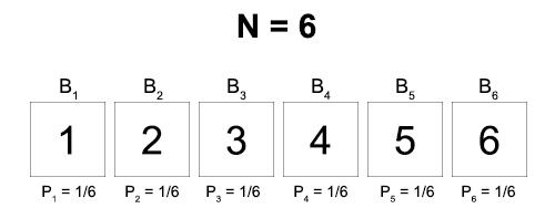
Here’s the setup. There are N boxes, and you know that a ball is in one of them. We’ll label the possible locations of the ball as:

B₁, B₂, B₃, … B_N
where B_n = “The ball is in box n”

The full state of our knowledge about which box the ball is in will be represented by a probability distribution.

(P₁, P₂, P₃, … P_N)
where P_n = the probability that the ball is in box n

Our ultimate goal is to uniquely prescribe an uncertainty measure S that will take in the distribution P and return a numerical value.

S(P₁, P₂, P₃, … P_N)

Our first assumption is that this function is continuous. When you make arbitrarily small changes to your distribution, you don’t get discontinuous jumps in your entropy. We’ll use this in a few minutes.

We’ll start with a simpler case than the general distribution – a uniform distribution, where the ball is equally likely to be in any of the N boxes.

For all n, P_n = 1/N

We’ll give the entropy of a uniform distribution a special name, labeled U for ‘uniform’:

S(1/N, 1/N, …, 1/N) = U(N)

Our next and final assumption is going to relate to the way that we combine our knowledge. In words, it will be that the uncertainty of a given distribution should be the same, regardless of how we represent the distribution. We’ll lay this out more formally in a moment.

Before that, imagine enclosing our boxes in M different containers, like this:

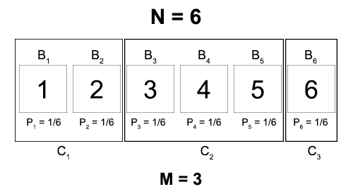
Now we can represent the same state of knowledge as our original distribution by specifying first the probability that the ball is in a given container, and then the probability that it is in a given box, given that it is in that container.

Q_n = probability that the ball is in container n
P_m|n = probability that the ball is in box m, given that it’s in container n

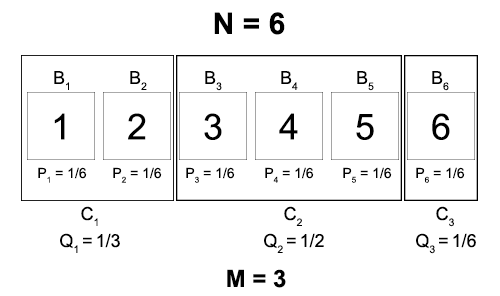
Notice that the value of each Q_n is just the number of boxes in the container divided by the total number of boxes. In addition, the conditional probability that the ball is in box m, given that it’s in container n, is just one over the number of boxes in the container. We’ll write these relationships as

Q_n = |C_n| / N
P_m|n = 1 / |C_n|

The point of all this is that we can now formalize our third assumption. Our initial state of knowledge was given by a single distribution P_n. Now it is given by two distributions: Q_n and P_m|n.

Since these represent the same amount of knowledge about which container the box is in, the entropy of each should be the same.

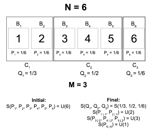
And in general:

Initial entropy = S(1/N, 1/N, …, 1/N) = U(N)
Final entropy = S(Q₁, Q₂, …, Q_M) + ∑_i Q_i · S(P_1|i, P_2|i, …, P_N|i)
= S(Q₁, Q₂, …, Q_M) + ∑_i Q_i · U(|C_i|)

The form of this final entropy is the substance of the uncertainty combination rule. First you compute the uncertainty of each individual distribution. Then you add them together, but weight each one by the probability that you encounter that uncertainty.

Why? Well, a conditional probability like P_m|n represents the probability that the ball is in box m, given that it’s in container n. You will only have to consider this probability if you discover that the ball is in container n, which happens with probability Q_n.

With this, we’re almost finished.

First of all, notice that we have the following equality:

S(Q₁, Q₂, …, Q_M) = U(N) – ∑_i [ Q_i · U(|C_i|) ]

In other words, if we determine the general form of the function U, then we will have uniquely determined the entropy S for any arbitrary distribution!

And we can determine the general form of the function U by making a final simplification: assume that the containers all contain an equal number of boxes.

This means that Q_n will be a uniform distribution over the M possible containers. And if there are M containers and N boxes, then this means that each container contains N/M boxes.

For all n, Q_n = 1/M and |C_n| = N/M

If we plug this all in, we get that:

S(1/M, 1/M, …, 1/M) = U(N) – ∑_i [1/M · U(N/M)]
U(M) = U(N) – U(N/M)
U(N/M) = U(N) – U(M)

There is only one continuous function that satisfies this equation, and it is the logarithm:

U(N) = K log(N) for some constant K

And we have uniquely determined the form of our entropy function, up to a constant factor K!

S(Q₁, Q₂, …, Q_M) = K log(N)  –  K ∑_i Q_i log(| C_i |)
= – K ∑_i Q_i log(| C_i |/N)
= – K ∑_i Q_i log(Q_i)

If we add as a third assumption that U(N) should be monotonically increasing with N (that is, more boxes means more uncertainty, not less), then we can also specify that K should be a positive constant.

The three basic assumptions from which we can find the form of the entropy:

1. S(P) is a continuous function of P.
2. S should assign the same uncertainty to different representations of the same information.
3. The entropy of a wide uniform distribution is greater than the entropy of a thin uniform distribution.