x^5 – x – 1

One of the strange and wonderful facts of mathematics is the general unsolvability of quintic polynomials. If you haven’t heard about this, prepare to have your mind pleasantly blown. Most people memorize the quadratic equation, the general expression for the roots of any quadratic polynomial, in high school:

And even though very few people learn it in school, it turns out that we know a general solution to any cubic polynomial as well. It’s a little cumbersome to write, but just like the quadratic equation, it expresses the zeroes of any cubic polynomial as a function of its coefficients.

ax³ + bx² + cx + d = 0
x = (some big complicated function of a, b, c, and d)

And in fact we have a general solution for any quartic polynomial as well, even more cumbersome.

ax⁴ + bx³ + cx² + dx + e = 0
x = (some even bigger and more complicated function of a, b, c, d, and e)

Mathematicians struggled for a long time to find a general solution for the roots of quintic polynomials (ax⁵ + bx⁴ + cx³ + dx² + ex + f = 0). Eventually, some mathematicians began to suspect that no such general solution existed. And then in the first few decades of the 1800s, a few mathematicians put out proofs to that effect. The most complete of these proofs was provided by Évariste Galois before he died in a duel at the age of 20 (we really need a big Hollywood movie about Galois’ life).

I recently found a fantastic 15-minute video sketching the proof of the unsolvability of the quintic. The approach taken in this proof is different from any of the original proofs, and it’s much simpler in a bunch of ways.

Here’s the video:

And briefly, here’s a summary of the proof:

1. The roots of any quintic polynomial obviously depend on the coefficients of the polynomial.
2. If you imagine taking a particular quintic polynomial (ax⁵ + bx⁴ + cx³ + dx² + ex + f), and making small continuous changes in the coefficients (a, b, c, d, e, f), then the set of zeroes of this polynomial should make similar continuous changes.
3. If you move each coefficient in a loop in the complex plane, ending at the same value it started at, then you should end up with the same set of zeroes as you started with (the same set, by the way, which doesn’t guarantee that each solution ends at the same place it started).
4. However, moving each coefficient in a loop in the complex plane sometimes ends up with the solutions switching places. (Illustration below)
5. For any “ordinary” function of the coefficients (a function that can be written using a finite number of rational numbers and the symbols +, -, ×, /, exp(), log(), √, and so on), you can find loops that don’t cause the solutions to switch places.
6. But for some quintic polynomials, you can always finds one of these loops that does cause the roots to switch places.
7. So there are quintic polynomials whose roots cannot be written as any ordinary function of the coefficients (since you can find a loop that permutes the solutions of the quintic but don’t permute the values of any ordinary function).

There are obviously holes in this proof that need to be filled. (1) through (3) should be pretty self-explanatory. And (4) can be illustrated by thinking about functions that involve square roots… on the complex plane, taking a square root of an expression means halving the angle to the expression. So rotating an expression around the complex plane by 2π only ends up rotating its square root by π (and thus bringing it to a different point). Observe:

And in general, a function involving an nth root of some ordinary expression will take n rotations around the complex plane to return each solution to its starting point. Take a look for n = 3:

For (5), you can prove this by using commutator loops (which are formed from two smaller loops L₁ and L₂ by putting them together as follows: L₁ L₂ L₁^-1 L₂^-1). Ultimately, this works for expressions with roots in them because solutions switch places exactly when you circle the origin of the complex plane, and commutators circle the origin a net zero times. For expressions with one nested root, you actually need to use commutators of commutators (first to return the inner root to its starting value, and then to return the outer root to its starting value). And with two nested roots, you use commutators of commutators of commutators. And so on. In this way, you can construct a loop in the complex plane for any expression you construct from roots and ordinary functions that will bring all values back to their starting points.

And finally, (6) is a result of the structure of the permutation group on five elements (S₅). If you look at all commutators of permutations of five elements, you are looking at the commutator subgroup of S₅, which is A₅ (the set of even permutations of five elements). And the commutator subgroup of A₅ is just A₅ itself. This means that you can find always find some commutator, or some commutator of commutators, or some commutator of commutators of commutators, (and so on) that is not equal to the identity permutation! (After all, if all commutators of commutators of commutators ended up just being the identity permutation, then the group of commutators of commutators of commutators would just be the trivial group {e}. But we already know that the group of commutators of commutators of commutators is just the commutator subgroup of the commutator subgroup of the commutator subgroup of S₅. I.e. the commutator subgroup of A₅, which is A₅.

And that’s the proof! You can see the whole thing sketched out in much more detail here.

Now, notice that the conclusion was that there are quintic polynomials whose roots cannot be written as any ordinary function of the coefficients. Not that all quintic polynomials’ roots can’t be written as such. Obviously, there are some quintics whose solutions can be written easily. For example…

x⁵ – 1 = 0
Solutions: x = e^2πik/5 for k = 0, 1, 2, 3, 4

But there also exist many quintic polynomials whose roots just have no way of being finitely expressed through ordinary functions! An example of this is the real root of x⁵ – x – 1.

x⁵ – x – 1 = 0
at x ≈ 1.167304…

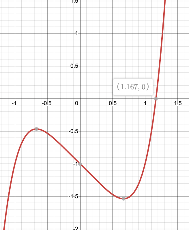
There is no way to write this number using a finite number of the symbols +, -, ×, /, exp(), log(), √, sin(), cos(), and rational numbers. And this is the case even though this number is an algebraic number! I don’t know if there’s a name for this category of “algebraic numbers that cannot be explicitly expressed using ordinary functions” but there should be.

Of course, you can define a function into existence that just returns the solutions of the quintic (which is what the Bring radical allows one to do). And you can also write the solution with ordinary functions if you’re allowed to use an infinity of them. For example, you can use a repeated fifth root:

x⁵ – x – 1 = 0
x⁵ = x + 1
x = (1 + x)^1/5
x = (1 + (1 + x)^1/5)^1/5
x = (1 + (1 + (1 + x)^1/5)^1/5)^1/5
x = (1 + (1 + (1 + (…))^1/5)^1/5)^1/5

But while an infinity of symbols suffices to express this 1.167304…, no finite number cuts it!