Can you compute all the countable ordinals?

One can live without knowing the ordinals, to be sure, but not as well.

Quote from this paper

What is an ordinal number? If you read my previous post, you might be convinced that an ordinal number is a particular type of set that contains all the ordinal numbers less than it. In particular, the ordinal 0 is the empty set, the ordinal 1 is the set {0}, the ordinal 2 is the set {0,1}, and so on. This is a fine way to think about ordinals, but there’s a much deeper view of them that I want to present in this post.

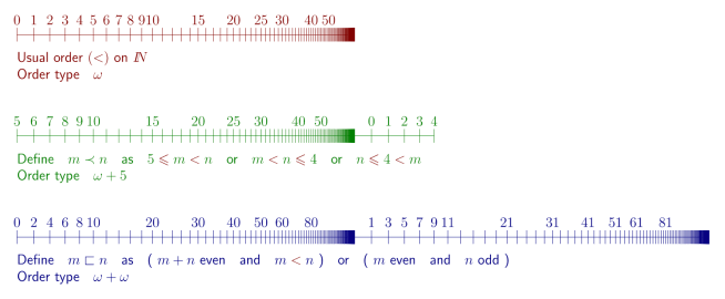
The fundamental concept is that of order types. Order types are to order-preserving bijections as cardinalities are to bijections. If you’ve seen pictures like these before, then they’re good to have in mind when you think about what order types are:

Let’s get into more detail about order types.

Take any two sets. If there is a bijection between them, then we say that they have the same cardinality. So we can think of each cardinal number as a class of sets, all in bijective correspondence with one another.

Take any two well-ordered sets. (Recall, a set is well-ordered if each of its subsets has a least element.) If there is an order-preserving bijection between them, then we say that the two sets have the same order type. So we can think of each ordinal number as a class of sets, all of the same order type.

For instance, the cardinal number “2” is the class of all sets with two elements (as all such sets are in bijective correspondence with one another). And the ordinal number “2” is the class of all well-ordered two-element sets. In particular, Von Neumann’s ordinal 2 = {0, 1} = {∅, {∅}} has this order type.

The finite cardinalities and finite order types line up nicely: any two well-ordered sets with the same finite cardinality are guaranteed to have the same order type. It’s in the realm of the infinite where order types and cardinalities come apart.

The cardinal number ℵ₀ is the class of all sets that can be put into bijective correspondence with the set of natural numbers ω. This includes the set of even numbers and the set of rational numbers. So how many order types are there of sets with cardinality ℵ₀?

Consider the following two ordered sets: X = {0 < 1 < 2 < 3 < …} and Y = {1 < 2 < 3 < … < 0}. They both have cardinality ℵ₀, but do they have the same order types? If so, then there must be a bijection f: X → Y such that f is order-preserving (for all a ∈ X and b ∈ X, if a < b then f(a) < f(b)). But what element of X is mapped to 0 in Y? In the set Y, 0 is larger than every element besides itself, but there is no element of X that has this property! So no, X and Y do not have the same order types.

X is the order type of ω (a countably infinite list of elements with no elements that have infinitely many predecessors), and Y is the order type of ω+1 (a countably infinite list of elements with a single element coming after all of them). This tells us that there are at least two different order types within the cardinality ℵ₀.

Can we construct an order on the set of natural numbers that has the same order type as ω+2? Well, all we need is for there to be two elements that are larger than all the rest. So we can write something like {2 < 3 < 4 < … < 0 < 1}. This generalizes easily to ω+n, for any finite n: {n+1 < n+2 < … < 0 < 1 < … < n} has the same order type as ω+n.

But now what about ω+ω, i.e. ω⋅2? To get a set of naturals with the same order type, we have to use a new trick. We need two countably infinite sequences of numbers that we can place beside one another. An easy way to accomplish this is by using the evens and odds: {0 < 2 < 4 < … < 1 < 3 < 5 < …}.

We can get an order on the naturals with the same order type as ω⋅2 + 1 by just choosing a single natural number to place after all the others. For instance: {2 < 4 < 6 < … < 1 < 3 < 5 < … < 0}. It should be easy to see how to get ω⋅2 + n for any finite n: just do {n < n+2 < n+4 < … < n+1 < n+3 < n+5 < … < 0 < 1 < 2 < … < n-1} And now how about ω⋅3?

(Try it out for yourself before reading on!)

To get ω⋅3, we need to place three countably infinite sequences of naturals side by side. For instance: {0 < 3 < 6 < … < 1 < 4 < 7 < … < 2 < 5 < 8 < …}.

For ω⋅4, we can use a similar trick: {0 < 4 < 8 < … < 1 < 5 < 9 < … < 2 < 6 < 10 < … < 3 < 7 < 11 < …}. Again, we can quite easily generalize this to ω⋅n for any finite n: {0 < n < 2n < … < 1 < n+1 < 2n+1 < … < 2 < n+2 < 2n+2 < … < … < n-1 < 2n-1 < 3n-1 < …}. But how about ω⋅ω? How do we deal with ω²?

This is a fun exercise to try for yourself at home. Construct an order on the set of natural numbers that has the same order type as ω². Then try to generalize the trick to get ω³, ω⁴, and ωⁿ for any finite n.

Next construct an order on the naturals with the same order type as ω^ω! Can you do it for ω^ω^ω? And ω^ω^ω^…? One thing that should become clear is that the larger an ordinal you’re dealing with, the harder it becomes to construct an order on the naturals with the same order type. The natural question is: is it always possible to do this type of construction, or do we at some point run out of clever tricks to use to get to higher and higher countable ordinals?

Well, if an ordinal α is countable, then it is a well-ordered set with the same cardinality as the naturals. So there always exists some order that can be placed on the naturals to mimic the order type of α. But is this order always computable?

We call an order on the naturals computable if there’s some Turing machine which takes as input two naturals x and y and outputs whether x < y according to this order. We call an order type computable if there’s some computable order on the naturals with that order type. The standard order (0 < 1 < 2 < 3 < …) is computable, and it’s easy to see how to compute all the other orders we’ve discussed so far. But are ALL the countable order types computable?

The wonderful and strange answer is no. There are countable order types that are uncomputable! There must exist orders on the naturals with such order types, but these orders are so immensely complicated and strange that they cannot be defined by ANY Turing machine! Here’s a quick and easy proof of this. (The next three paragraphs are the coolest and most important part of this whole post, so pay attention!)

Turn your mind back to Von Neumann’s construction of the ordinals, according to which each ordinal was exactly the set of all smaller ordinals. More technically, a set α is a Von Neumann ordinal iff α is well ordered with respect to ∈ AND every element of α is also a subset of α. Consider now the set of all countable ordinals. It can be seen that this set is itself an ordinal. Can it be a countable ordinal? No, because if it were then it would have to be an element of itself! (This is not allowed in ZFC by the axiom of regularity.) This means that there are uncountably many countable ordinals.

Ok, so far so good. Now we just observe that there are only countably many Turing machines. So there are only countably many Turing machines that compute orders on the naturals. And therefore there are only countably many computable ordinals.

Putting this together, we see that there are uncountably many uncomputable countable order types (say that sentence out loud). After all, there are uncountably many countable ordinals, and only countably many computable ordinals!

And if there’s only countably many computable ordinals, then there’s some countable Von Neumann ordinal consisting of the set of all computable ordinals! This set couldn’t possibly be computable, because then it would be contained within itself. So it’s the smallest uncomputable ordinal! This set is called the Church-Kleene ordinal. Its order type is literally so convoluted and complex that no Turing machine can compute it!