I ended the last post by saying that the solution to the problem of overfitting all relied on the concept of a model. So what is a model? Quite simply, a model is just a set of functions, each of which is a candidate for the true distribution that generates the data.
Why use a model? If we think about a model as just a set of functions, this seems kinda abstract and strange. But I think it can be made intuitive, and that in fact we reason in terms of models all the time. Think about how physicists formulate their theories. Laws of physics have two parts: First they specify the types of functional relationships there are in the world. And second, they specify the value of particular parameters in those functions. This is exactly how a model works!
Take Newton’s theory of gravity. The fundamental claim of this theory is that there is a certain functional relationship between the quantities a (the acceleration of an object), M (the mass of a nearby object), and r (the distance between the two objects): a ~ M/r2. To make this relationship precise, we need to include some constant parameter G that says exactly what this proportionality is: a = GM/r2.
So we start off with a huge set of probability distributions over observations of the accelerations of particles (one for each value of G), and then we gather data to see which value of G is most likely to be right. Einstein’s theory of gravity was another different model, specifying a different functional relationship between a, M, and r and involving its own parameters. So to compare Einstein’s theory of gravity to Newton’s is to compare different models of the phenomenon of gravitation.
When you start to think about it, the concept of a model is an enormous one. Models are ubiquitous, you can’t escape from them. Many fancy methods in machine learning are really just glorified model selection. For instance, a neural network is a model: the architecture of the network specifies a particular functional relationship between the input and the output, and the strengths of connections between the different neurons are the parameters of the model.
So. What are some methods for assessing predictive accuracy of models? The first one we’ll talk about is a super beautiful and clever technique called…
Cross Validation
The fundamental idea of cross validation is that you can approximate how well a model will do on the next data point by evaluating how the model would have done at predicting a subset of your data, if all it had access to was the rest of your data.
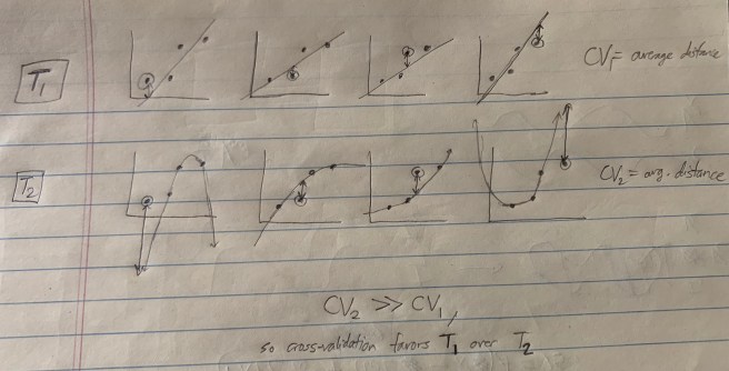
I’ll illustrate this with a simple example. Suppose you have a data set of four points, each of which is a tuple of two real numbers. Your two models are T1: that the relationship is linear, and T2: that the relationship is quadratic.
What we can do is go through each data point, selecting each in order, train the model on the non-selected data points, and then evaluate how well this trained model fits the selected data point. (By training the model, I mean something like “finding the curve within the model that best fits the non-selected data points.”) Here’s a sketch of what this looks like:
There are a bunch of different ways of doing cross validation. We just left out one data point at a time, but we could have left out two points at a time, or three, or any k less than the total number of points N. This is called leave-k-out cross validation. If we partition our data by choosing a fraction of it for testing, then we get what’s called n-fold cross validation (where 1/n is the fraction of the data that is isolated for testing).
We also have some other choices besides how to partition the data. For instance, we can choose to train our model via a Likelihoodist procedure or a Bayesian procedure. And we can also choose to test our model in various ways, by using different metrics for evaluating the distance between the testing set and the trained model. In leave-one-out cross validation (LOOCV), a pretty popular method, both the training and testing procedures are Likelihoodist.
Now, there’s a practical problem with cross-validation, which is that it can take a long time to compute. If we do LOOCV with N data points and look at all ways of leaving out one data point, then we end up doing N optimization procedures (one for each time you train your model), each of which can be pretty slow. But putting aside practical issues, for thinking about theoretical rationality, this is a super beautiful technique.
Next we’ll move on to…
Bayesian Model Selection!
We had Bayesian procedures for evaluating individual functions. Now we can go full Bayes and apply it to models! For each model, we assess the posterior probability of the model given the data using Bayes’ rule as usual:

Now… what is the prior Pr(M)? Again, it’s unspecified. Maybe there’s a good prior that solves overfitting, but it’s not immediately obvious what exactly it would be.
But there’s something really cool here. In this equation, there’s a solution to overfitting that pops up not out of the prior, but out of the LIKELIHOOD! I explain this here. The general idea is that models that are prone to overfitting get that way because their space of functions is very large. But if the space of functions is large, then the average prior on each function in the model must be small. So larger models have, on average, smaller values of the term Pr(f | M), and correspondingly (via 
So even without saying anything about the prior, we can see that Bayesian model selection provides a potential antidote to overfitting. But just like before, we have the practical problem that computing Pr(M | D) is in general very hard. Usually evaluating Pr(D | M) involves calculating a really complicated many-dimensional integral, and calculating many-dimensional integrals can be very computationally expensive.
Might we be able to find some simple unbiased estimator of the posterior Pr(M | D)? It turns out that yes, we can. Take another look at the equation above.
Since 

If we assume that P(D | f) is twice differentiable in the model parameters and that Pr(f) behaves roughly linearly around the maximum likelihood function, we can approximate this as:

f* is the maximum likelihood function within the model, and k is the the number of parameters of the model (e.g. k = 2 for a linear model and k = 3 for a quadratic model).
\We can make this a little neater by taking a logarithm and defining a new quantity: the Bayesian Information Criterion.
![argmax_M [ Pr(M | D) ] \\~\\ = argmax_M [ Pr(D | M) Pr(M) ] \\~\\ \approx argmax_M [ \frac {Pr(D | f^*(D))} {\sqrt{N}}^k Pr(M)] \\~\\ = argmax_M [ \log(Pr(M)) + \log (Pr(D | f^*(D)) - \frac{k}{2} \log(N) ] \\~\\ = argmin_M [ BIC - \log Pr(M) ]](https://s0.wp.com/latex.php?latex=argmax_M+%5B+Pr%28M+%7C+D%29+%5D+%5C%5C%7E%5C%5C++%3D+argmax_M+%5B+Pr%28D+%7C+M%29+Pr%28M%29+%5D+%5C%5C%7E%5C%5C++%5Capprox+argmax_M+%5B+%5Cfrac+%7BPr%28D+%7C+f%5E%2A%28D%29%29%7D%C2%A0%7B%5Csqrt%7BN%7D%7D%5Ek+Pr%28M%29%5D+%5C%5C%7E%5C%5C++%3D+argmax_M+%5B+%5Clog%28Pr%28M%29%29+%2B+%5Clog+%28Pr%28D+%7C+f%5E%2A%28D%29%29+-+%5Cfrac%7Bk%7D%7B2%7D+%5Clog%28N%29+%5D+%5C%5C%7E%5C%5C++%3D+argmin_M+%5B+BIC+-+%5Clog+Pr%28M%29+%5D+&bg=eeeeee&fg=666666&s=0&c=20201002)

Thus, to maximize the posterior probability of a model M is roughly the same as to minimize the quantity BIC – log Pr(M).
If we assume that our prior over models is constant (that is, that all models are equally probable at the outset), then we just minimize BIC.
Bayesian Information Criterion
Notice how incredibly simple this expression is to evaluate! If all we’re doing is minimizing BIC, then we only need to find the maximum likelihood function f*(D), assess the value of Pr(D | f*), and then penalize this quantity with the factor k/2 log(N)! This penalty scales in proportion to the model complexity, and thus helps us avoid overfitting.
We can think about this as a way to make precise the claims above about Bayesian Model Selection penalizing overfitting in the likelihood. Remember that minimizing BIC made sense when we assumed a uniform prior over models (and therefore when our prior doesn’t penalize overfitting). So even when we don’t penalize overfitting in the prior, we still end up getting a penalty! This penalty must come from the likelihood.
Some more interesting facts about BIC:
- It is approximately equal to the minimum description length criterion (which I haven’t discussed here)
- It is only valid when N >> k. So it’s not good for small data sets or large models.
- It the truth is contained within your set of models, then BIC will select the truth with probability 1 as N goes to infinity.
Okay, stepping back. We sort of have two distinct clusters of approaches to model selection. There’s Bayesian Model Selection and the Bayesian Information Criterion, and then there’s Cross Validation. Both sound really nice. But how do they compare? It turns out that in general they give qualitatively different answers. And in general, the answers you get using cross validation tend to be more predictively accurate that those that you get from BIC/BMS.
A natural question to ask at this point is: BIC was a nice simple approximation to BMS. Is there a corresponding nice simple approximation to cross validation? Well first we must ask: which cross validation? Remember that there was a plethora of different forms of cross validation, each corresponding to slightly different criterion for evaluating fits. We can’t assume that all these methods give the same answer.
Let’s choose leave-one-out cross validation. It turns out that yes, there is a nice approximation that is asymptotically equivalent to LOOCV! This is called the Akaike information criterion.
Akaike Information Criterion
First, let’s define AIC:

Like always, k is the number of parameters in M and f* is chosen by the Likelihoodist approach described in the last post.
What you get by minimizing this quantity is asymptotically equivalent to what you get by doing leave-one-out cross validation. Compare this to BIC:

There’s a qualitative difference in how the parameter penalty is weighted! BIC is going to have a WAY higher complexity penalty than AIC. This means that AIC should in general choose less simple models than BIC.
Now, we’ve already seen one reason why AIC is good: it’s a super simple approximation of LOOCV and LOOCV is good. But wait, there’s more! AIC can be derived as an unbiased estimator of the Kullback-Leibler divergence DKL.
What is DKL? It’s a measure of the information theoretic distance of a model from truth. For instance, if the true generating distribution for a process is f, and our model of this process is g, then DKL tells us how much information we lose by using g to represent f. Formally, DKL is:

Notice that to actually calculate this quantity, you have to already know what the true distribution f is. So that’s unfeasible. BUT! AIC gives you an unbiased estimate of its value! (The proof of this is complicated, and makes the assumptions that N >> k, and that the model is not far from the truth.)
Thus, AIC gives you an unbiased estimate of which model is closest to the truth. Even if the truth is not actually contained within your set of models, what you’ll end up with is the closest model to it. And correspondingly, you’ll end up getting a theory of the process that is very similar to how the process actually works.
There’s another version of AIC that works well for smaller sample sizes and larger models called AICc.

And interestingly, AIC can be derived as an approximation to Bayesian Model Selection with a particular prior over models. (Remember earlier when we showed that 

There’s a lot more to be said from here. This is only a short wade into the waters of statistical inference and model selection. But I think this is a good place to stop, and I hope that I’ve given you a sense of the philosophical richness of the various different frameworks for inference I’ve presented here.
