A mathematician is asked to design a table. He first designs a table with no legs. Then he designs a table with infinitely many legs. He spend the rest of his life generalizing the results for the table with N legs (where N is not necessarily a natural number).
A key feature of mathematics that makes it so variously fun or irritating (depending on who you are) is the tendency to abstract away from an initially practically useful question and end up millions of miles from where you started, talking about things that bear virtually no resemblance whatsoever to the topic you started with.
This gives rise to quotes like Feynman’s “Physics is to math what sex is to masturbation” and jokes like the one above.
I want to take you down one of these little rabbit holes of abstraction in this post, starting with factorials.
The definition of the factorial is the following:
N factorial = N! = N ∙ (N – 1) ∙ (N – 2) ∙ (…) ∙ 3 ∙ 2 ∙ 1
This function turns out to be mightily useful in combinatorics. The basic reason for this comes down to the fact that there are N! different ways of putting together N distinct objects into a sequence. The factorial also turns out to be extremely useful in probability theory and in calculus.
Now, the lover of abstraction looks at the factorial and notices that it is only defined for positive integers. We can say that 5! = 5 ∙ 4 ∙ 3 ∙ 2 ∙ 1 = 120, but what about something like ½!, or (-√2)!? Enter the Gamma function!
The Gamma function is one of my favorite functions. It’s weird and mysterious, and tremendously useful in a whole bunch of very different areas. Here’s the general definition:
𝚪(n) = ∫ xn e-x dx
(The integral should be taken from 0 to ∞, but I can’t figure out how to get WordPress to allow me to do this. Also, this is actually technically the Gamma function displaced by 1, but the difference won’t become important here.)
This function is the natural generalization of the factorial function, and we can prove it in just a few lines:
𝚪(n) = ∫ xn e-x dx
= ∫ n xn – 1 e-x dx
= n 𝚪(n – 1)
𝚪(0) = ∫ e-x dx = 1
This is sufficient to prove that 𝚪(n) is equal to n! for all integer values of n, since these two statements uniquely determine the values of the factorials of all positive integers.
n! = n ∙ (n – 1)!
0! = 1
The Gamma function generalizes the factorial not just to all real numbers, but to complex numbers. Not only can you say what ½! and (-√2)! are, you can say what i! is! Here are some of the values of the Gamma function:
(-½)! = √π
½! = √π/2
√2 ! ≈ -3.676
i! ≈ .5 – .15 i
The proof of the first two of these identities is nice, so I’ll lay it out briefly:
(-½)! = ∫ e-x/√x dx
= 2 ∫ e-u∙u du
= √π
(½)! = ½ (-½)! = √π/2
We can go further and deduce the values of the factorials of (3/2, 5/2, …) by just applying the definition of the factorial.
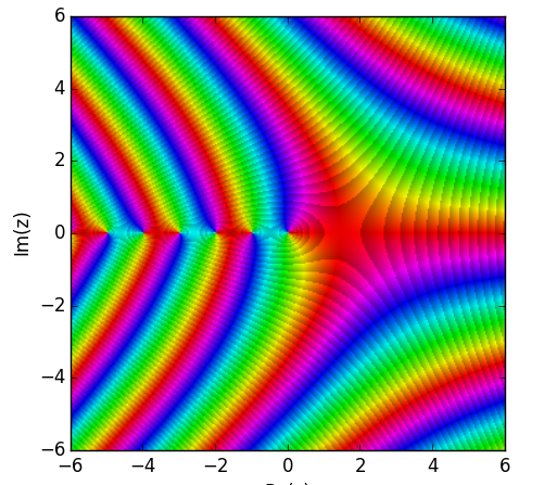
The function is also beautiful when plotted in the complex plane. Here’s a graph where the color corresponds to the complex value of the Gamma function.
At this point, one can feel that we are already lost in abstraction. Perhaps we had initially thought of the factorial as the quantity that tells you about the possible number of permutations of N distinct symbols. But what does it mean to say that there are about -3.676 ways of permuting √2 items, or (.5 – .15 i) ways of permuting an imaginary number of items?
To further frustrate our intuitions, the value of the Gamma function turns out to be undefined at every negative integer. (Some sense can be made of this by realizing that (-1)! is just 0!/0 = 1/0, which is undefined).

Often in times like these, it suits us to switch our intuitive understanding of the factorial to something that does generalize more nicely. Looking at the factorial in the context of probability theory can be helpful.
In statistical mechanics, it is common to describe distributions over events that individually have virtually zero probability of happening, but of which there are virtually infinite opportunities for them to happen, by a Poisson distribution.
An example of this might be a very unlikely radioactive decay. Suppose that the probability p of a single atom decaying is virtually zero, but the number N of atoms in the system you’re studying is virtually infinite ∞, and yet these balance in such a way that the product p∙N = λ is a finite and manageable number.
The Poisson distribution naturally arises as the answer to the question: What is the probability that N atoms decay in a period of time? The form of the distribution is:
P(n) = λn e-λ / n!

We can now use this to imagine a generalization for a process that doesn’t have to be discrete.
Say we are studying the amount of energy emitted in a system where individual emissions have virtually 0 probability but there are a virtually infinite amount of ways for the energy to be emitted. If the energy can take on any real value, then our distribution requires us to talk about the value of n! for arbitrary real n.
Anyway, let’s put aside the attempt to intuitively ground the Gamma function and talk about an application of this to calculus.
Calculus allows us to ask about the derivative of a function, the integral, the second derivative, the 15th derivative, and etc. Lovers of abstraction naturally began to ask questions like: “What’s the ½th derivative of a function? Are there imaginary derivatives?”
This opened the field known as fractional calculus.
Here’s a brief example of how we might do this.
The first derivative D of xn is n xn – 1
The second derivative D2 of xn is n∙(n – 1) ∙ xn – 2
The kth derivative Dk of xn is n! / (n – k)! ∙ xn – k
But we know how to generalize this to any non-integer value, because we know how to generalize the factorial function!
So, for instance, the ½th derivative of x turns out to be:
D½[x] = 1! / ½! ∙ x½
= 2/√π ∙ √x
Now, what we’ve presented is an identity that only applies to functions that look like xn. The general definition for a fractional derivative (or integral) is more complicated, but also uses the Gamma function.
What could it mean to talk about the fractional-derivative of a function? Intuitively, derivatives line up with slopes of curves, second derivatives are slopes of slopes, et cetera. What is a half-derivative of a curve?
I have no way to make intuitive sense of this, although fractional derivatives do tend to line up with our intuitive expectations for what an interpolation between functions should look like.

I’d be interested to know if there are types of functions whose fractional derivatives don’t have this property of smooth transitioning between the ordinary derivatives. Also, I could imagine a generalization of the Taylor approximation, where instead of aligning the integer derivatives of a function, we align all rational derivatives of the function, or all real-valued derivatives from 0 to 1.
The natural next step in this abstraction is to talk about functional calculus, where we can talk about not only arbitrary powers of derivatives, but arbitrary functions of derivatives. In this way we could talk about the logarithm or the sine of a derivative or an integral. But we’ll end the journey into abstraction here, as this ventures into territories that are foreign to me.
