How to draw lambda diagrams

If you don’t want spoilers for my puzzle a few days ago, don’t read ahead!

I think lambda diagrams are extremely cool, and haven’t seen any detailed description on how they work online. I’ll start by showing some very simple examples of lambda diagrams, and then build up to more complicated ones.

First of all, what are lambda diagrams? They are pictorial representations of lambda expressions, and hence count as a pictorial system for a large portion of mathematics. I will assume that you understand how lambda calculus works for this post, and if you aren’t familiar then you can do no better than this video for a basic introduction.

The Basics

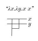
Let’s start simple: the lambda expression for “True”: λx.λy.x

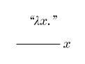
Each time we see a new bound variable, we draw a horizontal line to represent that variable. So parsing from left to right, we start with a horizontal line for x.

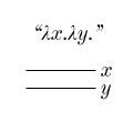
Next is “λy.“, so we insert another horizontal line for y (below the first horizontal line).

Next we have an x in the function body, which we represent by a vertical line leaving the x line:

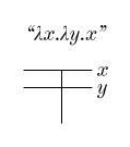
And there we have it, the lambda diagram for True!

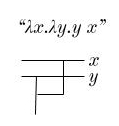
Now let’s look at False: λx.λy.y

We start the same way as before, with two horizontal lines for our variables x and y:

But now we have a y in our function body, not an x. So we draw our vertical line leaving the y line instead of the x line:

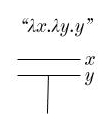
And that’s the diagram for False! The actual diagram needn’t have the labels “x” and “y” in it, because our convention that we draw lines for new variables below existing horizontal lines uniquely specifies which lines stand for which variables.

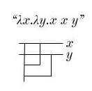
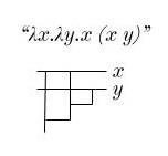
Let’s now do a slightly more complicated function: λx.λy.y x

As before, we start with our two variables, x and y.

Now we have a y in the function body, so we add a vertical line leaving the y bar:

Next is an x, which is being fed as input to the y. We draw this as follows:

Two things have happened here: First I’ve moved the original vertical line for y over to the left to make space. Next, I’ve represented “feeding x to y as input” as a line leaving the x bar and terminating at the vertical line for y.

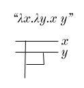
Take a guess what λx.λy.x y would look like!

…

…

…

Here it is:

Next, let’s look at λx.λy.x x y (which is incidentally the “or” function).

We start with the introduction of the variables x and y.

Next, an x:

And another x:

And finally a y:

Notice that this y connects below the first connection, to the original branch. What would it mean if it were connected to the second branch?

As you can see, this would indicate that y is first fed to x, and then the result of THAT is fed to x.

With these principles, you should now be able to draw out diagrams for much more complicated lambda expressions. Try this one: λx.λy.λz.z (y x) (y z x) x

…

…

…

Here it is!

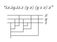
Make sure that this makes sense before moving on!

Lambda Expressions within Lambda Expressions

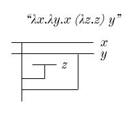
Next, we’ll look at how to deal with lambda expressions that contain new lambda expressions within their function body. Here’s a simple example: λx.λy.x (λz.z) y

Everything up until the third λ is the same as always:

Now, to deal with our new variable z, we draw a new horizontal line. But importantly, this horizontal line comes after the vertical line for the x that has already been used!

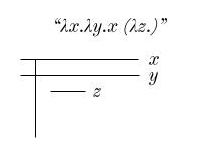
After the “λz.” we have a “z“, so we draw a line from the z bar to our original vertical line leaving x.

And finally, after all of this we feed y to the original vertical line:

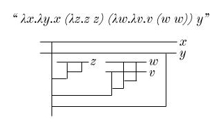
Try this one: λx.λy.x (λz.z z) (λw.λv.v (w w)) y

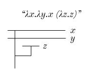
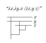
And here’s another one, where the inside function uses outside variables: λx.λy.x (λz.y z)

Alright, the final category you need to know to understand how to draw any lambda diagram whatsoever is…

Function Application

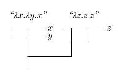
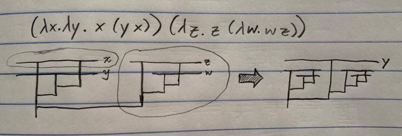
Suppose we have the lambda expression (λx.λy.x) (λz.z z). We first draw the lambda diagrams for each of the two component expressions side by side:

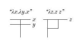
And now we simply attach the second to the first, indicating that the entire second lambda expression is fed as input to the first!

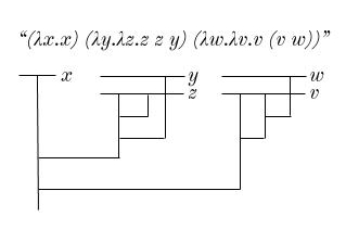
Here’s another example for you to try: (λx.x) (λy.λz.z z y) (λw.λv.v (v w))

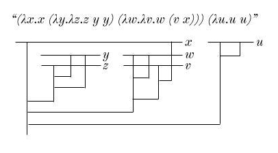
And one more example, this one using all the tricks we’ve seen so far: (λx.x (λy.λz.z y y) (λw.λv.w (v x))) (λu.u u)

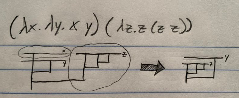
Beta Reduction

The final thing to know about lambda diagrams is how to actually do computations with them. The basic idea is that when we have one lambda diagram fed as input to another, we can substitute the “input” diagram for each vertical line leaving the topmost horizontal bar, and then erase this bar. Let’s look at some examples:

You can also do function application within larger lambda diagrams. Take a look at the following example, which is a calculation that shows that the successor of zero is one:

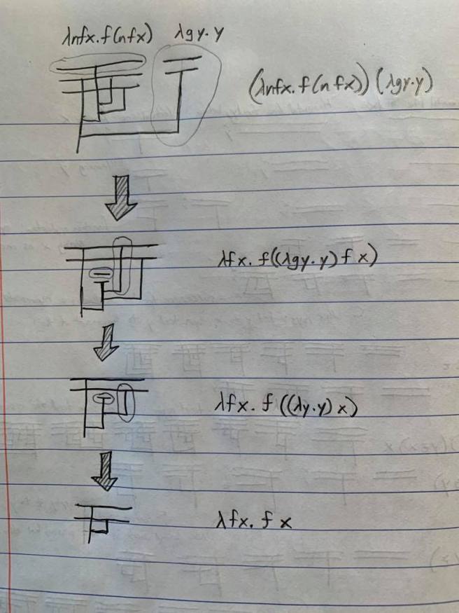
The first beta reduction here is just like the previous ones we’ve seen. But the second one does a substitution within the main lambda expression, as does the third. This works in much the same way as the earlier reductions we saw, the primary difference being that references to variables outside the scope of the function being applied must be maintained. You can see this in the final step above, where we remove the line representing the variable y, and attach the line connecting to it to the line representing the variable x.

Now for the fun part! I’ve found some great animations of calculations using lambda diagrams on Youtube. Each of them is using just the rules I’ve described above, nothing more! And I must say that the music is delightful. Take a look!

Beautiful!