Part 1: Quantum Computing in a Nutshell
Part 2: More on quantum gates
Part 3: Deutch-Josza Algorithm
Part 4: Grover’s algorithm
The quantum gate Uf was featured centrally in both of the previous algorithms I presented. Remember what it does to a qubit in state |x⟩, where x ∈ {0, 1}N:
![]()
I want to show here that this gate can be constructed from a simpler more intuitive version of a quantum oracle. This will also be good practice for getting a deeper intuition about how quantum gates work.
This will take three steps.
1. Addition Modulo 2
First we need to be able implement addition modulo 2 of two single qubits. This operation is defined as follows:

An implementation of this operation as a quantum gate needs to return two qubits instead of just one. A simple choice might be:
![]()


2. Oracle
Next we’ll need a straight-forward implementation of the oracle for our function f as a quantum gate. Remember that f is a function from {0, 1}N → {0, 1}. Quantum gates must have the same number of inputs and outputs, and f takes in N bits and returns only a single bit, so we have to improvise a little. A simple implementation is the following:


In other words, we start with N qubits encoding the input to x, as well as a “blank” qubit that starts as |0⟩. Then we leave the first N qubits unchanged, and encode the value of f(x) in the initially blank qubit.
3. Flipping signs
Finally, we’ll use a clever trick. Let’s take a second look at the ⊕ gate.
Suppose we start with
![]()
Then we get:

Let’s consider both cases, f(x) = 0 and f(x) = 1.

Also we can notice that we can get the state |y⟩ by applying a Hadamard gate to a qubit in the state |1⟩. Thus we can draw:

Putting it all together
We combine everything we learned so far in the following way:
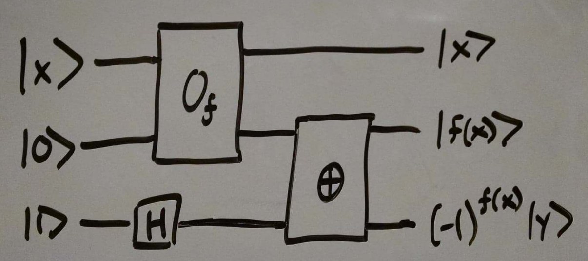
![]()
If we now ignore the last two qubits, as they were only really of interest to us for the purposes of building Uf , we get:
![]()
And there we have it! We have built the quantum gate Uf that we used in the last two posts.


2 thoughts on “Building the quantum oracle”