This post is about the relationship between entropy and relative entropy. This relationship is subtle but important – purely maximizing entropy (MaxEnt) is not equivalent to Bayesian conditionalization except in special cases, while maximizing relative entropy (ME) is. In addition, the justifications for MaxEnt are beautiful and grounded in fundamental principles of normative epistemology. Do these justifications carry over to maximizing relative entropy?
To a degree, yes. We’ll see that maximizing relative entropy is a more general procedure than maximizing entropy, and reduces to it in special cases. The cases where MaxEnt gives different results from ME can be interpreted through the lens of MaxEnt, and relate to an interesting distinction between commuting and non-commuting observations.
So let’s get started!
We’ll solve three problems: first, using MaxEnt to find an optimal distribution with a single constraint C1; second, using MaxEnt to find an optimal distribution with constraints C1 and C2; and third, using ME to find the optimal distribution with C2 given the starting distribution found in the first problem.
Part 1
Problem: Maximize – ∫ P logP dx with constraints
∫ P dx = 1
∫ C1[P] dx = 0
∂P ( – P1 logP1 + (α + 1) P1 + βC1[P1] ) = 0
– logP1 + α + β C1’[P1] = 0
Part 2
Problem: Maximize – ∫ P logP dx with constraints
∫ P dx = 1
∫ C1[P] dx = 0
∫ C2[P] dx = 0
∂P ( – P2 logP2 + (α’ + 1) P2 + β’C1[P2] + λ C2[P2] ) = 0
– logP2 + α’ + β’ C1’[P2] + λ C2’[P2] = 0
Part 3
Problem: Maximize – ∫ P log(P / P1) dx with constraints
∫ P dx = 1
∫ C2[P] dx = 0
∂P ( – P3 logP3 + P3 logP1 + (α’’ + 1)P3 + λ’ C2[P3] ) = 0
– logP3 + α’’ + logP1 + λ’ C2’[P3] = 0
– logP3 + α’’ + α + β C1’[P1] + λ’ C2’[P3] = 0
– logP3 + α’’’ + β C1’[P1] + λ’ C2’[P3] = 0
We can now compare our answers for Part 2 to Part 3. These are the same problem, solved with MaxEnt and ME. While they are clearly different solutions, they have interesting similarities.
MaxEnt
– logP2 + α’ + β’ C1’[P2] + λ C2’[P2] = 0
∫ P2 dx = 1
∫ C1[P2] dx = 0
∫ C2[P2] dx = 0
ME
– logP3 + α’’’ + β C1’[P1] + λ’ C2’[P3] = 0
∫ P3 dx = 1
∫ C1[P1] dx = 0
∫ C2[P3] dx = 0
The equations are almost identical. The only difference is in how they treat the old constraint. In MaxEnt, the old constraint is treated just like the new constraint – a condition that must be satisfied for the final distribution.
But in ME, the old constraint is no longer required to be satisfied by the final distribution! Instead, the requirement is that the old constraint be satisfied by your initial distribution!
That is, MaxEnt takes all previous information, and treats it as current information that must constrain your current probability distribution.
On the other hand, ME treats your previous information as constraints only on your starting distribution, and only ensures that your new distribution satisfy the new constraint!
When might this be useful?
Well, say that the first piece of information you received, C1, was the expected value of some measurable quantity. Maybe it was that x̄ = 5.
But if the second piece of information C2 was an observation of the exact value of x, then we clearly no longer want our new distribution to still have an expected value of x̄. After all, it is common for the expected value of a variable to differ from the exact value of x.
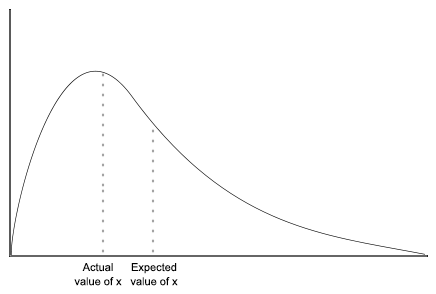
Once we have found the exact value of x, all previous information relating to the value of x is screened off, and should no longer be taken as constraints on our distribution! And this is exactly what ME does, and MaxEnt fails to do.
What about a case where the old information stays relevant? For instance, an observation of the values of a certain variable is not ‘cancelled out’ by a later observation of another variable. Observations can’t be un-observed. Does ME respect these types of constraints?
Yes!
Observations of variables are represented by constraints that set the distribution over those variables to delta-functions. And when your old distribution contains a delta function, that delta function will still stick around in your new distribution, ensuring that the old constraint is still satisfied.
Pold ~ δ(x – x’)
implies
Pnew ~ δ(x – x’)
The class of observations that are made obsolete by new observations are called non-commuting observations. They are given this name because for such observations, the order in which you process the information is essential. Observations for which the order of processing doesn’t matter are called commuting observations.
In summation: maximizing relative entropy allows us to take into account subtle differences in the type of evidence we receive, such as whether or not old data is made obsolete by new data. And mathematically, maximizing relative entropy is equivalent to maximizing ordinary entropy with whatever new constraints were not included in your initial distribution, as well as an additional constraint relating to the value of your old distribution. While the old constraints are not guaranteed to be satisfied by your new distribution, the information about them is preserved in the form of the prior distribution that is a factor in the new distribution.
