Part 3 of the series on quantum computing.
Part 1: Quantum Computing in a Nutshell
Part 2: More on quantum gates

Okay, now that we’re familiar with qubits and some basic quantum gates, we’re ready to jump into quantum algorithms. First will be the Deutch-Josza algorithm, famous for its exponential speedup.

The problem to solve: You are handed a function f from {0,1}^N to {0,1}, and guaranteed that it is either balanced or constant. A balanced function outputs an equal number of 0s and 1s across all inputs, and a constant function outputs all 0s or all 1s. For instance, if N = 3:

f₁ is balanced, and f₂ is constant.

You are given an oracle that allows you to query f on an input of your choice. Your goal is to find out if f is balanced or constant with as few queries to the oracle as possible.

Let’s first figure out the number of queries classically required to solve this problem.

If f is balanced, then the minimum amount of queries required to determine that it is not constant is two – a 0 and a 1. And the worst case is that f is constant. In this case, we can only be sure it is not balanced by searching through half of all possible inputs, plus one. (For instance, we might get the series of outputs 0, 0, 0, 0, 0.)

So, since the number of possible inputs is 2^N, the number of queries is between 2 and 2^N-1 + 1. The average case thus involves roughly 2^N-2 queries.

How about if we try to go about solving this problem with a quantum computers? How many queries to the oracle need we perform in order to determine if the function is balanced or constant?

Just one!

It turns out that there exists an algorithm that uses the oracle a single time, and always determines with 100% confidence whether f is balanced or constant.

Let’s prove it.

The algorithm uses only two different gates: the Hadamard gate H, and the quantum version of the oracle gate.

We’ll call the oracle gate U_f. Acting on the qubit state |x⟩, it returns (-1)^f(x)|x⟩. That is, it flips the sign of the state if and only if evaluating f on the input x outputs 1. Otherwise it leaves the state of the qubits unchanged. So we have:

In addition, we will use the general N-qubit Hadamard gate H^⊗N. We discussed how to get the matrix for the 2-qubit Hadamard gate last time. The general form of the Hadamard gate is:

(You can prove this by showing it’s true for N=1, and then showing that if it’s true for N, then it’s true for N+1.)

Without further ado, here is the Deutch-Josza algorithm:

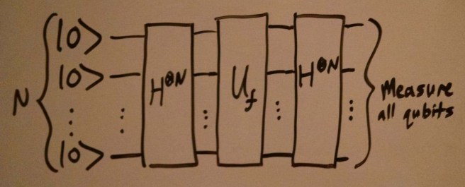
In words, you start with all N qubits in the state |00…0⟩. Then you apply H^⊗N to all of them. Then you apply U_f, and finally H^⊗N again.

Upon measurement, if you find the qubits in the state |00…0⟩, then f is a constant function. If you find them in any other state, then f is guaranteed to be a balanced function.

Why is this so? Let’s prove it by tracking the states through each step.

At first, the state is |00…0⟩. After applying the Hadamard gate, we get:

In words, the qubit enters a uniform superposition over all possible states.

Now, applying U_f to the new state, we get:

And finally, applying the Hadamard gate to this state, we get:

For the purposes of this algorithm, we’re really only interested in the amplitude of the |00…0⟩ state. This amplitude is simply:

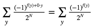
What we want to show is that the square of this amplitude is 0 if f is balanced and 1 if f is constant. (I.e. the probability of observing |00…0⟩ is 0% for a balanced function and 100% for a constant function). Let’s look at both cases in turn.

Case 1: f is constant

If f is constant, than all the terms in the sum are the same: either 1/2^N or -1/2^N. Since there are 2^N values for y to be summed over, the amplitude is either +1 or -1. And since the probability is the amplitude squared, this probability is guaranteed to be 100%!

Case 2: f is balanced

If f is balanced, then there are an equal number of 1/2^N terms and -1/2^N terms. I.e. every 1/2^N term cancels out a -1/2^N term. Thus, the amplitude is zero, and so is the probability!

—

In conclusion, we’ve now seen how a quantum computer can take a problem that can only be classically solved with an average of 2^N-2 queries, and solves it with exactly 1 query. I.e. quantum algorithms can provide exponential speedups over classical algorithms!

Looking carefully at the inner workings of this algorithm, you can get a clue as to how it achieves this speedup. The key is in the ability to superpose a single qubit into multiple observable states. This allowed us to apply our oracle operator to all possible inputs at once, in exactly one step.

Somebody that believed in the many-worlds interpretation of quantum mechanics would say that when we put our qubit into superposition, we were creating 2^N worlds, each of which contained a different possible input value. Then we leveraged this exponential number of worlds for our computational benefit, applying the operation in all the worlds at once before collapsing the superposition back to one single world with the final Hadamard gate.

It’s worth making a historical note here. David Deutsch was one of the two people that discovered this algorithm, which was the first example where a quantum computer would be able to surpass the ordinary limits on classical computers. He is also a hardcore proponent of the many-worlds interpretation, and has stated that the fact that quantum computers can do more than classical computers is strong evidence for this interpretation. His argument is that the only possible explanation for quantum computers surpassing the classical limits is that some of the computation is being offloaded into other universes.

Anyway, next we’ll look at a more famous algorithm, Grover’s algorithm. This one only provides a quadratic (not exponential) speed up. However, it solves a more useful problem: how to search through an unsorted list to find a particular item. See you next time!

Next: Grover’s algorithm