Iterated Simpson’s Paradox

December 29, 2017February 8, 2018 ~ squarishbracket ~ 4 Comments

In the last post, we saw how statistical reasoning can go awry in Simpson’s paradox, and how causal reasoning can rescue us. In this post, we’ll be generalizing the idea behind the paradox and producing arbitrarily complex versions of it.

The main idea behind Simpson’s paradox is that conditioning on an extra variable can sometimes reverse dependencies.

In our example in the last post, we saw that one treatment for kidney stones worked better than another, until we conditioned on the kidney stone’s size. Upon conditioning, the sign of the dependence between treatment and recovery changed, so that the first treatment now looked like it was less effective than the other.

We explained this as a result of a spurious correlation, which we represented with ‘paths of dependence’ like so:

But we can do better than just one reversal! With our understanding of causal models, we are able to generate new reversals by introducing appropriate new variables to condition upon.

Our toy model for this will be a population of sick people, some given a drug and some not (D), and some who recover and some who do not (R). If there are no spurious correlations between D and R, then our diagram is simply:

Iter Simpson's 0

Now suppose that we introduce a spurious correlation, wealth (W). Wealthy people are more likely to get the drug (let’s say that this occurs through a causal intermediary of education level E), and are more likely to recover (we’ll suppose that this occurs through a casual intermediary of nutrition level of diet N).

Now we have the following diagram:

Iter Simpson's 1

Where there was only previously one path of dependency between D and R, there is now a second. This means that if we observe W, we break the spurious dependency between D and R, and retain the true causal dependence.

Iter Simpson's 1 all paths Iter Simpson's 1 broken.png

This allows us one possible Simpson’s paradox: by conditioning upon W, we can change the direction of the dependence between D and R.

But we can do better! Suppose that your education level causally influences your nutrition. This means that we now have three paths of dependency between D and R. This allows us to cause two reversals in dependency: first by conditioning on W and second by conditioning on N.

Iter Simpson's 2 all paths.png Iter Simpson's 2 broke 1 Iter Simpson's 2 broke 2

And we can keep going! Suppose that education does not cause nutrition, but both education and nutrition causally impact IQ. Now we have three possible reversals. First we condition on W, blocking the top path. Next we condition on I, creating a dependence between E and N (via explaining away). And finally, we condition on N, blocking the path we just opened. Now, to discern the true causal relationship between the drug and recovery, we have two choices: condition on W, or condition on all three W, I, and N.

Iter Simpson's 3 all paths Iter Simpson's 3 cond WI Iter Simpson's 3 cond WIN

As might be becoming clear, we can do this arbitrarily many times. For example, here’s a five-step iterated Simpson paradox set-up:

Big iter simpson

The direction of dependence switches when you condition on, in this order: A, X, B’, X’, C’. You can trace out the different paths to see how this happens.

Part of the reason that I wanted to talk about the iterated Simpson’s paradox is to show off the power of causal modeling. Imagine that somebody hands you data that indicates that a drug is helpful in the whole population, harmful when you split the population up by wealth levels, helpful when you split it into wealth-IQ classes, and harmful when you split it into wealth-IQ-education classes.

How would you interpret this data? Causal modeling allows you to answer such questions by simply drawing a few diagrams!

Next we’ll move into one of the most significant parts of causal modeling – causal decision theory.

Previous: Simpson’s paradox

Next: Causal decision theory

Causal decision theory

December 29, 2017February 1, 2018 ~ squarishbracket ~ 2 Comments

Previous: Iterated Simpson’s Paradox

We’ll now move on into slightly new intellectual territory, that of decision theory.

While what we’ve previously discussed all had to do with questions about the probabilities of events and causal relationships between variables, we will now discuss questions about what the best decision to make in a given context is.

***

Decision theory has two ingredients. The first is a probabilistic model of different possible events that allows an agent to answer questions like “What is the probability that A happens if I do B?” This is, roughly speaking, the agent’s beliefs about the world.

The second ingredient is a utility function U over possible states of the world. This function takes in propositions, and returns the value to a particular agent of that proposition being true. This represents the agent’s values.

So, for instance, if A = “I win a million dollars” and B = “Somebody cuts my ear off”, U(A) will be a large positive number, and U(B) will be a large negative number. For propositions that an agent feels neutral or apathetic about, the utility function assigns them a value of 0.

Different decision theories represent different ways of combining a utility function with a probability distribution over world states. Said more intuitively, decision theories are prescriptions for combining your beliefs and your values in order to yield decisions.

A proposition that all competing decision theories agree on is “You should act to maximize your expected utility.” The difference between these different theories, then, is how they think that expected utility should be calculated.

“But this is simple!” you might think. “Simply sum over the value of each consequence, and weight each by its likelihood given a particular action! This will be the expected utility of that action.”

This prescription can be written out as follows:

Evidential Decision Theory.png

Here A is an action, C is the index for the different possible world states that you could end up in, and K is the conjunction of all of your background knowledge.

***

While this is quite intuitive, it runs into problems. For instance, suppose that scientists discover a gene G that causes both a greater chance of smoking (S) and a greater chance of developing cancer (C). In addition, suppose that smoking is known to not cause cancer.

Smoking Lesion problem

The question is, if you slightly prefer to smoke, then should you do so?

The most common response is that yes, you should do so. Either you have the cancer-causing gene or you don’t. If you do have the gene, then you’re already likely to develop cancer, and smoking won’t do anything to increase that chance.

And if you don’t have the gene, then you already probably won’t develop cancer, and smoking again doesn’t make it any more likely. So regardless of if you have the gene or not, smoking does not affect your chances of getting cancer. All it does is give you the little utility boost of getting to smoke.

But our expected utility formula given above disagrees. It sees that you are almost certain to get cancer if you smoke, and almost certain not to if you don’t. And this means that the expected utility of smoking includes the utility of cancer, which we’ll suppose to be massively negative.

Let’s do the calculation explicitly:

EU(S) = U(C & S) * P(C | S) + U(~C & S) * P(~C| S)
= U(C & S) << 0
EU(~S) = U(~S & C) * P(C | ~S) + U(~S & ~C) * P(~C | ~S)
= U(~S & ~C) ~ 0

Therefore we find that EU(~S) >> EU(S), so our expected utility formula will tell us to avoid smoking.

The problem here is evidently that the expected utility function is taking into account not just the causal effects of your actions, but the spurious correlations as well.

The standard way that decision theory deals with this is to modify the expected utility function, switching from ordinary conditional probabilities to causal conditional probabilities.

Causal Decision Theory.png

You can calculate these causal conditional probabilities by intervening on S, which corresponds to removing all its incoming arrows.

Smoking Lesion problem mutilated

Now our expected utility function exactly mirrors our earlier argument – whether or not we smoke has no impact on our chance of getting cancer, so we might as well smoke.

Calculating this explicitly:

EU(S) = U(S & C) * P(C | do S) + U(S & ~C) * P(~C | do S)
= U(S & C) * P(C) + U(S & ~C) * P(~C)
EU(~S) = U(~S & C) * P(C | do ~S) + U(S & ~C) * P(~C | do S)
= U(~S & C) * P(C) + U(~S & ~C) * P(~C)

Looking closely at these values, we can see that EU(S) must be greater than EU(~S), regardless of the value of P(C).

***

The first expected utility formula that we wrote down represents the branch of decision theory called evidential decision theory. The second is what is called causal decision theory.

We can roughly describe the difference between them as that evidential decision theory looks at possible consequences of your decisions as if making an external observation of your decisions, while causal decision theory looks at the consequences of your decisions as if determining your decisions.

EDT treats your decisions as just another event out in the world, while CDT treats your decisions like causal interventions.

Perhaps you think that the choice between these is obvious. But Newcomb’s problem is a famous thought experiment that famously splits people along these lines and challenges both theories. I’ve written about it here, but for now will leave decision theory for new topics.

Previous: Iterated Simpson’s Paradox

Next: Causality for philosophers

Free will and decision theory

December 29, 2017February 1, 2018 ~ squarishbracket ~ 5 Comments

This post is about one of the things that I’ve been recently feeling confused about.

In a previous post, I described different decision theories as different algorithms for calculating expected utility. So for instance, the difference between an evidential decision theorist and a causal decision theorist can be expressed in the following way:

EDT vs CDT

What I am confused about is that each decision theory involves a choice to designate some variables in the universe as “actions”, and all the others as “consequences.” I’m having trouble making a principled rule that tells us why some things can be considered actions and others not, without resorting to free will talk.

So for example, consider the following setup:

There’s a gene G in some humans that causes them to have strong desires for candy (D). This gene also causes low blood sugar (B) via a separate mechanism. Eating lots of candy (E) causes increased blood sugar. And finally, people have self-control (S), which help them not eat candy, even if they really desire it.

We can represent all of these relationships in the following diagram.

Free will.png

Now we can compare how EDT and CDT will decide on what to do.

If EDT looks at the expected utility of eating candy vs not eating candy, they’ll find both a negative dependence (eating candy makes a low blood sugar less likely), and a positive dependence (eating candy makes it more likely that you have the gene, which makes it more likely that you have a low blood sugar).

Let’s suppose that the positive dependence outweighs the low dependence, so that EDT ends up seeing that eating candy makes it overall more likely that you have a low blood sugar.

P(B | E) > P(B)

What does the CDT calculate? Well, they look at the causal conditional probability P(B | do E). In other words, they calculate their probabilities according to the following diagram.

Free will CDT

Now they’ll see only a single dependence between eating candy (E) and having a low blood sugar (B) – the direct causal dependence. Thus, they end up thinking that eating candy makes them less likely to have a low blood sugar.

P(B | do E) < P(B)

This difference in how they calculate probabilities may lead them to behave differently. So, for instance, if they both value having a low blood sugar much more than eating candy, then the evidential decision theorist will eat the candy, and the causal decision theorist will not.

Okay, fine. This all makes sense. The problem with this is, both of them decided to make their decision on the basis of what value of E maximizes expected utility. But this was not their only choice!

They could instead have said, “Look, whether or not I actually eat the candy is not under my direct control. That is, the actual movement of my hand to the candy bar and the subsequent chewing and swallowing. What I’m controlling in this process is my brain state before and as I decide to eat the candy. In other words, what I can directly vary is the value of S – whether or not the self-controlled part of my mind tells me to eat the candy or not. The value of E that ends up actually obtaining is then a result of my choice of the value of S.”

If they had thought this way, then instead of calculating EU(E) and EU(~E), they would calculate EU(S) and EU(~S), and go with whichever one maximizes expected utility.

But now we get a different answer than before!

In particular, CDT and EDT are now looking at the same diagram, because when the causal decision theorist intervenes on the value of S, there are no causal arrows for them to break. This means that they calculate the same probabilities.

P(B | S) = P(B | do S)

And thus get the same expected utility values, resulting in them behaving the same way.

Furthermore, somebody else might argue “No, don’t be silly. We don’t only have control over S, we have control over both S, and E.” This corresponds to varying both S and E in our expected utility calculation, and choosing the optimal values. That is, they choose the actions that correspond to the max of the set { EU(S, E), EU(S, ~E), EU(~S, E), EU(~S, ~E) }.

Another person might say “Yes, I’m in control of S. But I’m also in control of D! That is, if I try really hard, I can make myself not desire things that I previously desired.” This person will vary S and D, and choose that which optimizes expected utility.

Another person will claim that they are in control of S, D, and E, and their algorithm will look at all eight combinations of these three values.

Somebody else might say that they have partial control over D. Another person might claim that they can mentally affect their blood sugar levels, so that B should be directly included in their set of “actions” that they use to calculate EU!

And all of these people will, in general, get different answers.

***

Some of these possible choices of the “set of actions” are clearly wrong. For instance, a person that says that they can by introspection change the value of G, editing out the gene in all of their cells, is deluded.

But I’m not sure how to make a principled judgment as to whether or not a person should calculate expected utilities varying S and D, varying just S, varying just E, and other plausible choices.

What’s worse, I’m not exactly sure how to rigorously justify why some variables are “plausible choices” for actions, and others not.

What’s even worse, when I try to make these types of principled judgments, my thinking naturally seems to end up relying on free-will-type ideas. So we want to say that we are actually in control of S, and in a sense we can’t really freely choose the value of D, because it is determined by our genes.

But if we extend this reasoning to its extreme conclusion, we end up saying that we can’t control any of the values of the variables, as they are all the determined results of factors that are out of our control.

If somebody hands me a causal diagram and tells me which variables they are “in control of”, I can tell them what CDT recommends them to do and what EDT recommends them to do.

But if I am just handed the causal diagram by itself, it seems that I am required to make some judgments about what variables are under the “free control” of the agent in question.

One potential way out of this is to say that variable X is under the control of agent A if, when they decide that they want to do X, then X happens. That is, X is an ‘action variable’ if you can always trace a direct link between the event in the brain of A of ‘deciding to do X’ and the actual occurrence of X.

Two problems that I see with this are (1) that this seems like it might be too strong of a requirement, and (2) that this seems to rely on a starting assumption that the event of ‘deciding to do X’ is an action variable.

On (1): we might want to say that I am “in control” of my desire for candy, even if my decision to diminish it is only sometimes effectual. Do we say that I am only in control of my desire for candy in those exact instances when I actually successfully determine their value? How about the cases when my decision to desire candy lines up with whether or not I desire candy, but purely by coincidence? For instance, somebody walking around constantly “deciding” to keep the moon in orbit around the Earth is not in “free control” of the moon’s orbit, but this way of thinking seems to imply that they are.

And on (2): Procedurally, this method involves introducing a new variable (“Decides X”), and seeing whether or not it empirically leads to X. After all, if the part of your brain that decides X is completely out of your control, then it makes as much sense to say that you can control X as to say that you can control the moon’s orbit. But then we have a new question, about how much this decision is under your control. There’s a circularity here.

We can determine if “Decides X” is a proper action variable by imagining a new variable “Decides (Decides X)”, and seeing if it actually is successful at determining the value of “Decides X”. And then, if somebody asks us how we know that “Decides (Decides X)” is an action variable, we look for a variable “Decides (Decides (Decides X))”. Et cetera.

How can we figure our way out of this mess?

Simpson’s paradox

December 29, 2017December 27, 2018 ~ squarishbracket ~ 4 Comments

Previous: Screening off and explaining away

A look at admission statistics at a college reveals that women are less likely to be admitted to graduate programs than men. A closer investigation reveals that in fact when the data is broken down into individual department data, women are more likely to be admitted than men. Does this sound impossible to you? It happened at UC Berkeley in 1973.

When two treatments are tested on a group of patients with kidney stones, Treatment A turns out to lead to worse recovery rates than Treatment B. But when the patients are divided according to the size of their kidney stone, it turns out that no matter how large their kidney stone, Treatment A always does better than Treatment B. Is this a logical contradiction? Nope, it happened in 1986!

What’s going on here? How can we make sense of this apparently inconsistent data? And most importantly, what conclusions do we draw? Is Berkeley biased against women or men? Is Treatment A actually more effective or less effective than Treatment B?

In this post, we’ll apply what we’ve learned about causal modeling to be able to answer these questions.

***

Quine gave the following categorization of types of paradoxes: veridical paradoxes (those that seem wrong but are actually correct), falsidical paradoxes (those that seem wrong and actually are wrong), and antinomies (those that are premised on common forms of reasoning and end up deriving a contradiction).

Simpson’s paradox is in the first category. While it seems impossible, it actually is possible, and it happens all the time. Our first task is to explain away the apparent falsity of the paradox.

Let’s look at some actual data on the recovery rates for different treatments of kidney stones.

	Treatment A	Treatment B
All patients	78% (273/350)	83% (289/350)

The percentages represent the number of patients that recovered, out of all those that were given the particular treatment. So 273 patients recovered out of the 350 patients given Treatment A, giving us 78%. And 289 patients recovered out of the 350 patients given Treatment B, giving 83%.

At this point we’d be tempted to proclaim that B is the better treatment. But if we now break down the data and divide up the patients by kidney stone size, we see:

	Treatment A	Treatment B
Small stones	93% (81/87)	87% (234/270)
Large stones	73% (192/263)	69% (55/80)

And here the paradoxical conclusion falls out! If you have small stones, Treatment A looks better for you. And if you have large stones, Treatment A looks better for you. So no matter what size kidney stones you have, Treatment A is better!

And yet, amongst all patients, Treatment B has a higher recovery rate.

Small stones: A better than B
Large stones: A better than B
All sizes: B better than A

I encourage you to check out the numbers for yourself, in case you still don’t believe this.

***

The simplest explanation for what’s going on here is that we are treating conditional probabilities like they are joint probabilities. Let’s look again at our table, and express the meaning of the different percentages more precisely.

	Treatment A	Treatment B
Small stones	P(Recovery \| Small stones & Treatment A)	P(Recovery \| Small stones & Treatment B)
Large stones	P(Recovery \| Large stones & Treatment A)	P(Recovery \| Large stones & Treatment B)
Everybody	P(Recovery \| Treatment A)	P(Recovery \| Treatment B)

Our paradoxical result is the following:

But this is no paradox at all! There is no law of probability that tells us:

There is, however, a law of probability that tells us:

And if we represented the data in terms of these joint probabilities (probability of recovery AND small stones given Treatment A, for example) instead of conditional probabilities, we’d find that the probabilities add up nicely and the paradox vanishes.

	Treatment A	Treatment B
Small stones	23% (81/350)	67% (234/350)
Large stones	55% (192/350)	16% (55/350)
All patients	78% (273/350)	83% (289/350)

It is in this sense that the paradox arises from improper treatment of conditional probabilities as joint probabilities.

***

This tells us why we got a paradoxical result, but isn’t quite fully satisfying. We still want to know, for instance, whether we should give somebody with small kidney stones Treatment A or Treatment B.

The fully satisfying answer comes from causal modeling. The causal diagram we will draw will have three variables, A (which is true if you receive Treatment A and false if you receive Treatment B), S (which is true if you have small kidney stones and false if you have large), and R (which is true if you recovered).

Our causal diagram should express that there is some causal relationship between the treatment you receive (A) and whether you recover (R). It should also show a causal relationship between the size of your kidney stone (S) and your recovery, as the data indicates that larger kidney stones make recovery less likely.

And finally, it should show a causal arrow from the size of the kidney stone to the treatment that you receive. This final arrow comes from the fact that more people with large stones were given Treatment A than Treatment B, and more people with small stones were given Treatment B than Treatment B.

This gives us the following diagram:

Simpson's paradox

The values of P(S), P(A | S), and P(A | ~S) were calculated from the table we started with. For instance, the value of P(S) was calculated by adding up all the patients that had small kidney stones, and dividing by the total number of patients in the study: (87 + 270) / 700.

Now, we want to know if P(R | A) > P(R | ~A) (that is, if recovery is more likely given Treatment A than given Treatment B).

If we just look at the conditional probabilities given by our first table, then we are taking into account two sources of dependency between treatment type and recovery. The first is the direct causal relationship, which is what we want to know. The second is the spurious correlation between A and R as a result of the common cause S.

Simpson's paradox paths

Here the red arrows represent “paths of dependency” between A and R. For example, since those with small stones are more likely to get treatment B, and are also more likely to recover, this will result in a spurious correlation between small stones and recovery.

So how we do we determine the actual non-spurious causal dependency between A and R?

Easy!

If we observe the value of S, then we screen A off from R through S! This removes the spurious correlation, and leaves us with just the causal relationship that we want.

Simpson's paradox broken

What this means is that the true nature of the relationship between treatment type and recovery can be determined by breaking down the data in terms of kidney stone size. Looking back at our original data:

Recovery rate	Treatment A	Treatment B
Small stones	93% (81/87)	87% (234/270)
Large stones	73% (192/263)	69% (55/80)
All patients	78% (273/350)	83% (289/350)

This corresponds to looking at the data divided up by size of stones, and not the data on all patients. And since for each stone size category, Treatment A was more effective than Treatment B, this is the true causal relationship between A and R!

***

A nice feature of the framework of causal modeling is that there are often multiple ways to think about the same problem. So instead of thinking about this in terms of screening off the spurious correlation through observation of S, we could also think in terms of causal interventions.

In other words, to determine the true nature of the causal relationship between A and R, we want to intervene on A, and see what happens to R.

This corresponds to calculating if P(R | do A) > P(R | do ~A), rather than if P(R | A) > P(R | ~A).

Intervention on A gives us the new diagram:

Simpson's paradox intervene

With this diagram, we can calculate:

And…

Now not only do we see that Treatment A is better than Treatment B, but we can have the exact amount by which it is better – it improves recovery chances by about 5%!

Next, we’re going to go kind of crazy with Simpson’s paradox and show how to construct an infinite chain of Simpson’s paradoxes.

Fantastic paper on all of this here.

Previous: Screening off and explaining away

Next: Iterated Simpson’s paradox

Screening off and explaining away

December 29, 2017February 8, 2018 ~ squarishbracket ~ 7 Comments

Previous: Correlation and causation

In this post, I’ll explain three of the most valuable tools for inference that arise naturally from causal modeling.

Screening off via causal intermediary
Screening off via common cause
Explaining away

First:

Suppose that the rain causes the sidewalk to get wet, and the sidewalk getting wet causes you to slip and break your elbow.

rain & slip & elbow.png

This means that if you know that it’s raining, then you know that a broken elbow is more likely. But if you also know that the sidewalk is wet, then learning whether or not it is raining no longer makes a broken elbow more likely. After all, the rain is only a useful piece of information for predicting broken elbows insofar as it allows you to infer sidewalk-wetness.

In other words, the information about sidewalk-wetness screens off the information about whether or not it is raining with respect to broken elbows. In particular, sidewalk-wetness screens off rain because it is a causal intermediary to broken elbows.

Second:

Suppose that being wealthy causes you to eat more nutritious food, and being wealthy also causes you to own fancy cars.

common cause.png

This means that if you see somebody in a fancy car, you know it is more likely that they eat nutritious food. But if you already knew that they were wealthy, then knowing that their car is fancy tells you no more about the nutritiousness of their diet. After all, the fanciness of the car is only a useful piece of information for predicting nutritious diets insofar as it allows you to infer wealth.

In other words, wealth screens off ownership of fancy cars with respect to nutrition. In particular, wealth screens off ownership of fancy cars because it is a common cause of nutrition and fancy car owning.

Third:

Suppose that being really intelligent causes you to get on television, and being really attractive causes you to get on television, but attractiveness and intelligence are not directly causally related.

smart & hot & tv.png

This means that in the general population, you don’t learn anything about somebody’s intelligence by assessing their attractiveness. But if you know that they are on television, then you do learn something about their intelligence by assessing their attractiveness.

In particular, if you know that somebody is on television, and then you learn that they are attractive, then it becomes less likely that they intelligent than it was before you learned this.

We say that in this scenario attractiveness explains away intelligence, given the knowledge that they are on television.

***

I want to introduce some notation that will allow us to really compactly describe these types of effects and visualize them clearly.

We’ll depict an ‘observed variable’ in a causal diagram as follows:

A>B>C with observed B

This diagram says that A causes B, B causes C, and the value of B is known.

In addition, we talked about the value of one variable telling you something about the value of another variable, given some information about other variables. For this we use the language of dependence.

To say, for example, that A and B are independent given C, we write:

(A ⫫ B) | C

And to say that A and B are dependent given C, we just write:

~(A ⫫ B) | C

With this notation, we can summarize everything I said above with the following diagram:

Screening off and explaining away

In words, the first row expresses dependent variables that become independent when conditioning on causal intermediaries. B screens off A from C as a causal intermediary.

The second expresses dependent variables that become independent when conditioning on common causes. B screens off A from C as a common cause.

And the third row expresses independent variables that become dependent when conditioning on common effects. A explains away C, given B.

***

Repeated application of these three rules allows you to determine dependencies in complicated causal diagrams. Let’s say that somebody gives you the following diagram:

Complex cause

First they ask you if E and F are going to be correlated.

We can answer this just by tracing causal paths through the diagram. If we look at all connected triples on paths leading from E to F and find that there is dependence between the end variables in each triple, then we know that E and F are dependent.

The path ECA is a causal chain, and C is not observed, so E and A are dependent along this path. Next, the path CAD is a common cause path, and the common cause (A) is not observed, thus retaining dependence again along the path. And finally, the path ADF is a causal chain with D unobserved, so A and F are dependent along the path.

So E and F are dependent.

Now your questioner tell you the value of D, and re-asks you if E and F are dependent.

Complex cause obs D

Now dependence still exists along the paths ECA and CAD, but the path ADF breaks the dependence. This follows from the rule in row 1: D is observed, so A is screened off from F. Since A is screened off, E is as well. This means that E and F are now independent.

Suppose they asked you if E and B were dependent before telling you the value of D. In this case, the dependence travels along ECA, and along CAD, but is broken along ADB by observation of D. This follows from our rule in row 3.

And if they asked you if E and B were dependent after telling you the value of D, then you would respond that they are dependent. Now the last leg of the path (ADB) is dependent, because A and B explain each other away.

The general ability to look at a complicated causal diagram is a valuable tool, and we will come back to it in the future.

Next, I’ll talk about one of my current favorite applications of causal diagrams: Simpson’s paradox!

Previous: Correlation and causation

Next: Simpson’s paradox

Societal Failure Modes

December 29, 2017March 15, 2018 ~ squarishbracket ~ Leave a comment

(Nothing original, besides potentially this specific way of framing the concepts. This post started off short and ended up wayyy too long, and I don’t have the proper level of executive control to make myself shorten it significantly. So sorry, you’re stuck with this!)

Noam Chomsky in a recent interview said about the Republican Party:

I mean, has there ever been an organization in human history that is dedicated, with such commitment, to the destruction of organized human life on Earth? Not that I’m aware of. Is the Republican organization – I hesitate to call it a party – committed to that? Overwhelmingly. There isn’t even any question about it.

And later in the same interview:

… extermination of the species is very much an – very much an open question. I don’t want to say it’s solely the impact of the Republican Party – obviously, that’s false – but they certainly are in the lead in openly advocating and working for destruction of the human species.

In Chomsky’s mind, members of the Republican Party apparently sit in dark rooms scheming about how best to destroy all that is good and sacred.

I just watched the most recent Star Wars movie, and was struck by a sense of some relationship between the sentiment being expressed by Chomsky here and a statement made by Supreme Leader Snoke:

The seed of the Jedi Order lives. As long as he does, hope lives within the galaxy. I thought you would be the one to snuff it out.

There’s a really easy pattern of thought to fall into, which is something like “When things go wrong, it’s because of evil people doing evil things.”

It’s a really tempting idea. It diagnoses our societal problems as a simple “good guys vs bad guys” story – easy to understand and to convince others of. And it comes with an automatic solution, one that is very intuitive, simple, and highly self-gratifying: “Get rid of the bad guys, and just let us good guys make all the decisions!”

I think that the prevalence of this sort of story in the entertainment industry gives us some sort of evidence of its memetic power as a go-to explanation for problems. Think about how intensely the movie industry is optimizing for densely packed megadoses of gratifying storylines, visual feasts, appealing characters, and all the rest. The degree to which two and a half hours can be packed with constant intense emotional stimulation is fairly astounding.

Given this competitive market for appealing stories, it makes sense that we’d expect to gain some level of insight into the types of memes that we are most vulnerable to by looking at those types of stories and plot devices that appear over and over again. And this meme in particular, the theme of “social problems are caused by evil people,” is astonishingly universal across entertainment.

***

That this meme is wrong is the first of two big insights that I’ve been internalizing more and more in the past year. These are:

When stuff goes wrong, or the world seems like it’s stuck in shitty and totally repairable ways, the only explanation is not evil people. In fact, this is often the least helpful explanation.
Talking about the “motives” of an institution can be extremely useful. These motives can overpower the motives of the individuals that make up that institution, making them more or less irrelevant. In this way, we can end up with a description of institutions with weird desires and inclinations that are totally distinct from those of the people that make them up, and yet the institutions are in charge of what actually happens in the world.

On the second insight first: this is a sense in which institutions can be very very powerful. It’s not just the sense of powerful that means “able to implement lots of large-scale policies and cause lots of big changes”. It’s more like “able to override the desires of individuals within your range of influence, manipulating and bending them to your will.”

I was talking to my sister and her fiancé, both law students, about the US judicial system, and Supreme Court justices in particular. I wanted to understand what it is that really constrains the decisions of these highest judicial authorities; what are the forces that result in Justice Ginsberg writing the particular decision that she ends up writing.

What they ended up concluding is that there are essentially no such external forces.

Sure, there are ways in which Supreme Court justices can lose their jobs in principle, but this has never actually happened. And Congress can and does sometimes ignore Supreme Court decisions on statutory issues, but this doesn’t generally give the Justices any less reason to write their decision any differently.

What guides Justice Ginsberg is what she believes is right – her ideology – and perhaps legacy. In other words, purely internal forces. I wanted to think of other people in positions that allow similar degrees of power in ability to enact social change, and failed.

The first sense of power as ‘able to cause lots of things to happen” really doesn’t align with the second sense of ‘free from external constraints on your decision-making‘. An autocratic ruler might be plenty powerful in terms of ability to decide economic policy or assassinate journalists or wage war on neighboring states, but is highly constrained in his decisions by a tight incentive structure around what allows him to keep doing these things.

On the other hand, a Supreme Court justice could have total power to do whatever she personally desires, but never do anything remarkable or make any significant long-term impact on society.

The fact that this is so rare – that we could only think of a single example of a position like this – tells us about the way that powerful institutions are able to warp and override the individual motivations of the humans that compose them.

The rest of this post is on the first insight, about the idea that social problems are often not caused by evil people. There are two general things to say about evil people:

I think that it’s often the case that “evil people” is a very surface-level explanation, able to capture some aspects of reality and roughly get at the problem, but not touching anywhere near the roots of the issue. One example of this may be when you ask people what the cause of the 2007 financial crisis was, and they go on about greedy bankers destroying America with their insatiable thirst for wealth.
While they might be landing on some semblance of truth there, they are really missing a lot of important subtlety in terms of the incentive structures of financial institutions, and how they led the bankers to behave in the way that they did. They are also very naturally led to unproductive “solutions” to the problems – what do we do, ban greed? No more bankers? Chuck capitalism? (Viva la revolución?) If you try to explain things on the deeper level of the incentive structures that led to “greedy banker” behavior, then you stand a chance of actually understanding how to solve the root problem and prevent it from recurring.
Appeals to “evil people” can only explain a small proportion of the actual problems that we actually see in the world. There are a massive number of ways in which groups of human beings, all good people not trying to cause destruction and chaos or extinguish the last lights of hope in the universe, can end up steering themselves into highly suboptimal and unfortunate states.

My main goal in this post is to try to taxonomize these different causes of civilizational failure.

Previously I gave a barebones taxonomy of some of the reasons that low-hanging policy fruits might be left unplucked. Here I want to give a more comprehensive list.

***

I think a useful way to frame these issues is in terms of Nash equilibria. The worst-case scenario is where there are Pareto improvements all around us, and yet none of these improvements correspond to worlds that are in a Nash equilibrium. These are cases where the prospect of improvement seems fairly hopeless without a significant restructuring of our institutions.

Slightly better scenarios are where we have improvements that do correspond to a world in a Nash equilibrium, but we just happen to be stuck in a worse Nash equilibrium. So to start with, we have:

The better world is not in a Nash equilibrium
The better world is in a Nash equilibrium

I think that failures of the first kind are very commonly made amongst bright-eyed idealists trying to imagine setting up their perfect societies.

These types of failures correspond to questions like “okay, so once you’ve set up your perfect world, how will you assure that it stays that way?” and can be spotted in plans that involve steps like “well, I’m just assuming that all the people in my world are kind enough to not follow their incentives down this obvious path to failure.”

Nash equilibria correspond to stable societal setups. Any societal setup that is not in a Nash equilibrium can fairly quickly be expected to degenerate into some actually stable societal set-up.

The ways in which a given societal set up fails to be stable can be quite subtle and non-obvious, which I suspect is why this step is so often overlooked by reformers that think they see obvious ways to improve the world.

One of my favorite examples of this is the make-up problem. It starts with the following assumptions: (1) makeup makes people more attractive (which they want to be), and (2) an individual’s attractiveness is valued relative to the individuals around them.

Let’s now consider two societies, a make-up free society and a makeup-ubiquitous society. In both societies, everybody’s relative attractiveness is the same, which means that nobody is better off or worse off in one society over another on the basis of their attractiveness.

But the society in which everybody wears makeup is worse for everybody, because everybody has to spend a little bit of their money buying makeup. In other words, the makeup-free world represents a Pareto improvement over the makeup-ubiquitous world.

What’s worse; the makeup-free world is not in a Nash equilibrium, and the makeup-ubiquitous society is!

We can see this by imagining a society that starts makeup-free, and looking at the incentives of an individual within that society. This individual only stands to gain by wearing makeup, because she becomes more attractive relative to everybody else. So she buys makeup. Everybody else reasons the same way, so the make-up free society quickly degenerates into its equilibrium version, the makeup-ubiquitous society.

Sure, she can see that if everybody reasoned this way, then she will be worse off (she would have spent her money and gained nothing from it). But this reasoning does not help her. Why? Because regardless of what everybody else does, she is still better off wearing makeup.

If nobody wears makeup, then her relative attractiveness rises if she wears makeup. And if everybody else wears makeup, then her relative attractiveness rises if she wears makeup. It’s just that it’s rising from a lower starting point.

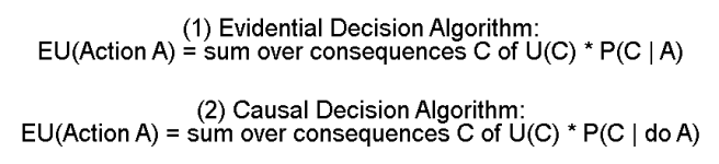
So no matter what society we start in, we end up in the suboptimal makeup-ubiquitous society. (I have to point out here that this is assuming a standard causal decision theory framework, which I think is wrong. Timeless decision theory will object to this line of reasoning, and will be able to maintain a makeup free equilibrium.)

We want to say “but just in this society assume that everybody is a good enough person to recognize the problem with makeup-wearing, and doesn’t do so!“

But that’s missing the entire point of civilization building – dealing with the fact that we will end up leaving non-Nash-equilibrium societal setups and degenerating in unexpected ways.

This failure mode arises because of the nature of positional goods, which are exactly what they sound like. In our example, attractiveness is a positional good, because your attractiveness is determined by looking at your position with respect to all other individuals (and yes this is a bit contrived and no I don’t think that attractiveness is purely positional, though I think that this is in part an actual problem).

To some degree, prices are also a positional good. If all prices fell tomorrow, then everybody would quickly end up with the same purchasing power as they had yesterday. And if everybody got an extra dollar to spend tomorrow, then prices would rise in response, the value of their money would decrease, and nobody would be better off (there are a lot of subtleties that make this not actually totally true, but let’s set that aside for the sake of simplicity).

Positional goods are just one example where we can naturally end up with our desired societies not being Nash equilibria.

The more general situation is just bad incentive structures, whereby individuals are incentivized to defect against a benevolent order, and society tosses and turns and settles at the nearest Nash equilibrium.

The better world is not a Nash equilibrium
- Positional goods
- Bad incentive structures
The better world is a Nash equilibrium

***

If the better world is in a Nash equilibrium, then we can actually imagine this world coming into being and not crumbling into a degenerate cousin-world. If a magical omniscient society-optimizing God stepped in and rearranged things, then they would likely stay that way, and we’d end up with a stable and happier world.

But there are a lot of reasons why all of us that are not magical society-optimizing Gods can do very little to make the changes that we desire. Said differently, there are many ways in which current Nash equilibria can do a great job of keeping us stuck in the existing system.

Three basic types of problems are (1) where the decision makers are not incentivized to implement this policy, (2) where valuable information fails to reach decision makers, and (3) where decision makers do have the right incentives and information, but fail because of coordination problems.

The better world is not a Nash equilibrium
- Positional goods
- Bad incentive structures
The better world is a Nash equilibrium
- You can’t reach it because you’re stuck in a lesser Nash equilibrium.
  - Lack of incentives in decision makers
  - Asymmetric information
  - Coordination problems

Lack of incentives in decision makers can take many forms. The most famous of these occurs when policies result in externalities. This is essentially just where decision-makers do not absorb some of the consequences of a policy.

Negative externalities help to explain why behaviors that are net negative to society exist and continue (resulting in things like climate change and overfishing, for example), and positive externalities help to explain why some behaviors that would be net positive for society are not happening.

An even worse case of misalignment of incentives would be where the positive consequences on society would be negative consequences on decision-makers, or vice-versa. Our first-past-the-post voting system might be an example of this – abandoning FPTP would be great exactly because it allows us to remove the current set of decision-makers and replace them with a better set. This would great for us, but not so great for them.

I’m not aware of a name for this class of scenarios, and will just call it ‘perverse incentives.’

I think that this is also where the traditional concept of “evil people” would lie – evil people are those whose incentives are dramatically misaligned. This could mean that they are apathetic towards societal improvements, but typically fiction’s common conception of villains is individuals actively trying to harm society.

Lack of liquidity is another potential source of absent incentives. This is where there are plenty of individuals that do have the right incentives, but there is not enough freedom for them to actually make significant changes.

An example of this could be if a bunch of individuals all had the same idea for a fantastic new app that would perform some missing social function, and all know how to make the app, but are barred by burdensome costs of actually entering the market and getting the app out there.

The app will not get developed and society will be worse off, as a result of the difficulty in converting good app ideas to cash.

Lack of incentives in decision makers
- Misalignment of incentives
  - Externalities
  - Perverse incentives
    - Evil people
  - Lack of liquidity

***

Asymmetric information is a well-known phenomenon that can lead societies into ruts. The classic example of this is the lemons problem. There are versions of asymmetric information problems in the insurance market, the housing market, the health care market and the charity market.

This deserves its own category because asymmetric information can bar progress, even when decision-makers have good incentives and important good policy ideas are out there.

Lack of incentives in decision makers
- Misalignment of incentives
  - Externalities
  - Perverse incentives
    - Evil people
  - Lack of liquidity
- Asymmetric information

And of course, there are coordination problems. The makeup example given earlier is an example of a coordination problem – if everybody could successfully coordinate and avoid the temptation of makeup, then they’d all end up better off. But since each individual is incentivized to defect, the coordination attempts will break down.

Coordination problems generally occur when you have multi-step or multi-factor decision processes. I.e. when the decision cannot be unilaterally made by a single individual, and must be done as a cooperative effort between groups of individuals operating under different incentive structures.

A nice clear example of this comes from Eliezer Yudkowsky, who imagines a hypothetical new site called Danslist, designed to be a competitor to Craigslist.

Danslist is better than Craigslist in every way, and everybody would prefer that it was the site in use. The problem is that Craigslist is older, so everybody is already on that site.

Buyers will only switch to Danslist if there are enough sellers there, and sellers will only switch to Danslist if there are enough buyers there. This makes the decision to switch to Danslist a decision that is dependent on two factors, the buyers and the sellers.

In particular, an N-factor market is one where there are N different incentive structures that must interact for action to occur. In N-factor markets, the larger N is, the more difficult it is to make good decisions happen.

This is really important, because when markets are stuck in this way, inefficiencies arise and people can profit off of the sub-optimality of the situation.

So Craigslist can charge more than Danslist, while offering a worse service, as long as this doesn’t provide sufficient incentive for enough people to switch over.

Yudkowsky also talks about Elsevier as an instance of this. Elsevier is a profiteer that captured several large and prestigious scientific journals and jacked up subscription prices. While researchers, universities, and readers could in principle just unanimously switch their publication patterns to non-Elsevier journals, this involves solving a fairly tough coordination problem. (It has happened a few times)

One solution to coordination problems is an ability to credibly pre-commit. So if everybody in the makeup-ubiquitous world was able to sign a magical agreement that truly and completely credibly bound their future actions in a way that they couldn’t defect from, then they could end up in a better world.

When individuals cannot credibly pre-commit, then this naturally results in coordination problems.

And finally, there are other weird reasons that are harder to categorize for why we end up stuck in bad Nash equilibria.

For instance, a system in which politicians respond to the wills of voters and are genuinely accountable to them seems like a system with a nicely aligned incentive structure.

But if for some reason, the majority of the public resists policies that will actually improve their lives, or push policies that will hurt them, then this system will still end up in a failure mode. Perhaps this failure mode is not best expressed as a Nash equilibrium, as there is a sense in which voters do have the incentive to switch to a more sensible view, but I will express it as such regardless.

This looks to me like what is happening with popular opinion about minimum wage laws.

Huge amounts of people support minimum wage laws, including those that may actually lose their jobs as the result of those laws. While I’m aware that there isn’t a strong consensus among economists as to the real effects of a moderate minimum-wage increase, it is striking to me that so many people are so convinced that it can only be net positive for them, when there is plenty of evidence that it may not be.

Another instance of this is the idea of “wage stickiness”.

This is the idea that employers are more likely to fire their workers than to lower their wages, resulting in an artificial “stickiness” to the current wages. The proposed reason for why this is so is that worker morale is hurt more by decreased wages than by coworkers being fired.

Sticky wages are especially bad when you take into account inflation effects. If an economy has an inflation rate of 10%, then an employer that keeps her employees’ wages constant is in effect cutting their wages by 10%. Even if she raises their wages by 5%, they’re still losing money!

And if the economy enters a recession, with say an inflation rate of -5%, then an employer will have to cut wages by 5% in order to stay at the market equilibrium. But since wages are sticky and her workers won’t realize that they are actually not losing any money despite the wage cut, she will be more likely to fire workers instead.

A friend described to me an interaction he had had with a coworker at a manufacturing plant. My friend had been recently hired in the same position as this man, and was receiving the minimum wage at 5 dollars an hour.

His coworker was telling him about how he was being paid so much, because he had been working there so many years and was constantly getting pay raises. He was mortified when he compared wages with my friend, and found that they were receiving the exact same amount.

Status quo bias is another important effect to keep in mind here. Individuals are likely to favor the current status quo, for no reason besides that it is the status quo. This type of effect can add to political inertia and further entrench society in a suboptimal Nash equilibrium.

I’ll just lump all of these effects in as “Stupidity & cognitive biases.”

***

I want to close by adding a third category that I’ve been starting to suspect is more important than I previously realized. This is:

The better world is in a Nash equilibrium, and you can reach it, and you will reach it, just WAIT a little bit.

I add this because I sometimes forget that society is a massive complicated beast with enormous inertia behind its existing structure, and that just because some favored policy of yours has not yet been fully implemented everywhere, this does not mean that there is a deep underlying unsolvable problem.

So, for instance, one time I puzzled for a couple weeks about why, given the apparently low cost of ending global poverty forever, it still exists.

Aren’t there enough politicians that are aware of the low cost? And aren’t they sufficiently motivated to pick up the windfall of public support and goodwill that they would surely get? (To say nothing of massively improving the world)

Then I watched Hans Rosling’s 2008 lecture “Don’t Panic” (which, by the way, should be required watching for everyone) and realized that global poverty is actually being ended, just slowly and gradually.

The UN set a goal in 2000 to completely end all world poverty by 2030. They’ve already succeeded in cutting it in half, and are five years ahead of their plan.

We’re on course to see the end of extreme poverty; it’ll just take a few more years. And after all, it should be expected that raising an entire segment of the world’s population above the poverty line will take some time.

So in this case, the answer to my question of “Why is this problem not being solved, if solutions exist?” was actually “Um, it is being solved, you’re just impatient.”

And earlier I wrote about overfishing and the ridiculously obvious solutions to the problem. I concluded by pessimistically noting that the fishing lobby has a significant influence over policy makers, which is why the problem cannot by solved.

While the antecedent of this is true, it is in fact the case that ITQ policies are being adopted in more and more fisheries, the Atlantic Northwest cod fisheries are being revived as a result of marine protection policies, and governments are making real improvements along this front.

This is a nice optimistic note to end on – the idea that not everything is a horrible unsolvable trap and that we can and do make real progress.

***

So we have:

The better world is not a Nash equilibrium
- Positional goods
- Bad incentive structures
The better world is a Nash equilibrium
- You can’t reach it because you’re stuck in a lesser Nash equilibrium.
  - Lack of incentives in decision makers
    - Misalignment of incentives
      - Externalities
      - Perverse incentives
      - Lack of liquidity
  - Asymmetric information
  - Coordination problems
    - Multi-factor markets
    - Multi-step decision processes
    - Inability to pre-commit
  - Stupidity & cognitive biases
- You can and will reach it, just be patient.

I don’t think that this overall layout is perfect, or completely encompasses all failure modes of society. But I suspect that it is along the right lines of how to think about these issues. I’ve had conversations where people will say things like “Society would be better if we just got rid of all money” or “If somebody could just remove all those darned Republicans from power, imagine how much everything would improved” or “If I was elected dictator-for-life, I could fix all the world’s problems.”

I think that people that think this way are often really missing the point. It’s dead easy to look at the world’s problems, find somebody or something to point at and blame, and proclaim that removing them will fix everything. But the majority of the work you need to do to actually improve society involves answering really hard questions like “Am I sure that I haven’t overlooked some way in which my proposed policy degenerates into a suboptimal Nash equilibrium? What types of incentive structures naturally arise if I modify society in this way? How could somebody actually make this societal change from within the current system?”

That’s really the goal of this taxonomy – is to try to give a sense of what the right questions to be asking are.

(More & better reading along these same lines here and here.)