Free will and decision theory

This post is about one of the things that I’ve been recently feeling confused about.

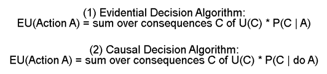
In a previous post, I described different decision theories as different algorithms for calculating expected utility. So for instance, the difference between an evidential decision theorist and a causal decision theorist can be expressed in the following way:

EDT vs CDT

What I am confused about is that each decision theory involves a choice to designate some variables in the universe as “actions”, and all the others as “consequences.” I’m having trouble making a principled rule that tells us why some things can be considered actions and others not, without resorting to free will talk.

So for example, consider the following setup:

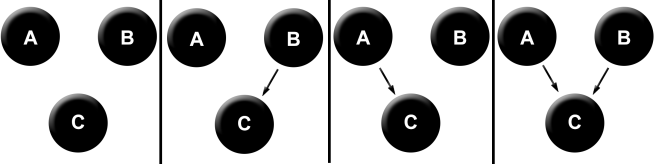
There’s a gene G in some humans that causes them to have strong desires for candy (D). This gene also causes low blood sugar (B) via a separate mechanism. Eating lots of candy (E) causes increased blood sugar. And finally, people have self-control (S), which help them not eat candy, even if they really desire it.

We can represent all of these relationships in the following diagram.

Free will.png

Now we can compare how EDT and CDT will decide on what to do.

If EDT looks at the expected utility of eating candy vs not eating candy, they’ll find both a negative dependence (eating candy makes a low blood sugar less likely), and a positive dependence (eating candy makes it more likely that you have the gene, which makes it more likely that you have a low blood sugar).

Let’s suppose that the positive dependence outweighs the low dependence, so that EDT ends up seeing that eating candy makes it overall more likely that you have a low blood sugar.

P(B | E) > P(B)

What does the CDT calculate? Well, they look at the causal conditional probability P(B | do E). In other words, they calculate their probabilities according to the following diagram.

Free will CDT

Now they’ll see only a single dependence between eating candy (E) and having a low blood sugar (B) – the direct causal dependence. Thus, they end up thinking that eating candy makes them less likely to have a low blood sugar.

P(B | do E) < P(B)

This difference in how they calculate probabilities may lead them to behave differently. So, for instance, if they both value having a low blood sugar much more than eating candy, then the evidential decision theorist will eat the candy, and the causal decision theorist will not.

Okay, fine. This all makes sense. The problem with this is, both of them decided to make their decision on the basis of what value of E maximizes expected utility. But this was not their only choice!

They could instead have said, “Look, whether or not I actually eat the candy is not under my direct control. That is, the actual movement of my hand to the candy bar and the subsequent chewing and swallowing. What I’m controlling in this process is my brain state before and as I decide to eat the candy. In other words, what I can directly vary is the value of S – whether or not the self-controlled part of my mind tells me to eat the candy or not. The value of E that ends up actually obtaining is then a result of my choice of the value of S.”

If they had thought this way, then instead of calculating EU(E) and EU(~E), they would calculate EU(S) and EU(~S), and go with whichever one maximizes expected utility.

But now we get a different answer than before!

In particular, CDT and EDT are now looking at the same diagram, because when the causal decision theorist intervenes on the value of S, there are no causal arrows for them to break. This means that they calculate the same probabilities.

P(B | S) = P(B | do S)

And thus get the same expected utility values, resulting in them behaving the same way.

Furthermore, somebody else might argue “No, don’t be silly. We don’t only have control over S, we have control over both S, and E.” This corresponds to varying both S and E in our expected utility calculation, and choosing the optimal values. That is, they choose the actions that correspond to the max of the set { EU(S, E), EU(S, ~E), EU(~S, E), EU(~S, ~E) }.

Another person might say “Yes, I’m in control of S. But I’m also in control of D! That is, if I try really hard, I can make myself not desire things that I previously desired.” This person will vary S and D, and choose that which optimizes expected utility.

Another person will claim that they are in control of S, D, and E, and their algorithm will look at all eight combinations of these three values.

Somebody else might say that they have partial control over D. Another person might claim that they can mentally affect their blood sugar levels, so that B should be directly included in their set of “actions” that they use to calculate EU!

And all of these people will, in general, get different answers.

***

Some of these possible choices of the “set of actions” are clearly wrong. For instance, a person that says that they can by introspection change the value of G, editing out the gene in all of their cells, is deluded.

But I’m not sure how to make a principled judgment as to whether or not a person should calculate expected utilities varying S and D, varying just S, varying just E, and other plausible choices.

What’s worse, I’m not exactly sure how to rigorously justify why some variables are “plausible choices” for actions, and others not.

What’s even worse, when I try to make these types of principled judgments, my thinking naturally seems to end up relying on free-will-type ideas. So we want to say that we are actually in control of S, and in a sense we can’t really freely choose the value of D, because it is determined by our genes.

But if we extend this reasoning to its extreme conclusion, we end up saying that we can’t control any of the values of the variables, as they are all the determined results of factors that are out of our control.

If somebody hands me a causal diagram and tells me which variables they are “in control of”, I can tell them what CDT recommends them to do and what EDT recommends them to do.

But if I am just handed the causal diagram by itself, it seems that I am required to make some judgments about what variables are under the “free control” of the agent in question.

One potential way out of this is to say that variable X is under the control of agent A if, when they decide that they want to do X, then X happens. That is, X is an ‘action variable’ if you can always trace a direct link between the event in the brain of A of ‘deciding to do X’ and the actual occurrence of X.

Two problems that I see with this are (1) that this seems like it might be too strong of a requirement, and (2) that this seems to rely on a starting assumption that the event of ‘deciding to do X’ is an action variable.

On (1): we might want to say that I am “in control” of my desire for candy, even if my decision to diminish it is only sometimes effectual. Do we say that I am only in control of my desire for candy in those exact instances when I actually successfully determine their value? How about the cases when my decision to desire candy lines up with whether or not I desire candy, but purely by coincidence? For instance, somebody walking around constantly “deciding” to keep the moon in orbit around the Earth is not in “free control” of the moon’s orbit, but this way of thinking seems to imply that they are.

And on (2): Procedurally, this method involves introducing a new variable (“Decides X”), and seeing whether or not it empirically leads to X. After all, if the part of your brain that decides X is completely out of your control, then it makes as much sense to say that you can control X as to say that you can control the moon’s orbit. But then we have a new question, about how much this decision is under your control.  There’s a circularity here.

We can determine if “Decides X” is a proper action variable by imagining a new variable “Decides (Decides X)”, and seeing if it actually is successful at determining the value of “Decides X”. And then, if somebody asks us how we know that “Decides (Decides X)” is an action variable, we look for a variable “Decides (Decides (Decides X))”. Et cetera.

How can we figure our way out of this mess?

Simpson’s paradox

Previous: Screening off and explaining away

A look at admission statistics at a college reveals that women are less likely to be admitted to graduate programs than men. A closer investigation reveals that in fact when the data is broken down into individual department data, women are more likely to be admitted than men. Does this sound impossible to you? It happened at UC Berkeley in 1973.

When two treatments are tested on a group of patients with kidney stones, Treatment A turns out to lead to worse recovery rates than Treatment B. But when the patients are divided according to the size of their kidney stone, it turns out that no matter how large their kidney stone, Treatment A always does better than Treatment B. Is this a logical contradiction? Nope, it happened in 1986!

What’s going on here? How can we make sense of this apparently inconsistent data? And most importantly, what conclusions do we draw? Is Berkeley biased against women or men? Is Treatment A actually more effective or less effective than Treatment B?

In this post, we’ll apply what we’ve learned about causal modeling to be able to answer these questions.

***

Quine gave the following categorization of types of paradoxes: veridical paradoxes (those that seem wrong but are actually correct), falsidical paradoxes (those that seem wrong and actually are wrong), and antinomies (those that are premised on common forms of reasoning and end up deriving a contradiction).

Simpson’s paradox is in the first category. While it seems impossible, it actually is possible, and it happens all the time. Our first task is to explain away the apparent falsity of the paradox.

Let’s look at some actual data on the recovery rates for different treatments of kidney stones.

Treatment A Treatment B
All patients 78% (273/350) 83% (289/350)

The percentages represent the number of patients that recovered, out of all those that were given the particular treatment. So 273 patients recovered out of the 350 patients given Treatment A, giving us 78%. And 289 patients recovered out of the 350 patients given Treatment B, giving 83%.

At this point we’d be tempted to proclaim that B is the better treatment. But if we now break down the data and divide up the patients by kidney stone size, we see:

Treatment A Treatment B
Small stones 93% (81/87) 87% (234/270)
Large stones 73% (192/263) 69% (55/80)

And here the paradoxical conclusion falls out! If you have small stones, Treatment A looks better for you. And if you have large stones, Treatment A looks better for you. So no matter what size kidney stones you have, Treatment A is better!

And yet, amongst all patients, Treatment B has a higher recovery rate.

Small stones: A better than B
Large stones: A better than B
All sizes: B better than A

I encourage you to check out the numbers for yourself, in case you still don’t believe this.

***

The simplest explanation for what’s going on here is that we are treating conditional probabilities like they are joint probabilities. Let’s look again at our table, and express the meaning of the different percentages more precisely.

Treatment A Treatment B
Small stones P(Recovery | Small stones & Treatment A) P(Recovery | Small stones & Treatment B)
Large stones P(Recovery | Large stones & Treatment A) P(Recovery | Large stones & Treatment B)
Everybody P(Recovery | Treatment A) P(Recovery | Treatment B)

Our paradoxical result is the following:

P(Recovery | Small stones & Treatment A) > P(Recovery | Small stones & Treatment B)
P(Recovery | Large stones & Treatment A) > P(Recovery | Large stones & Treatment B)
P(Recovery | Treatment A) < P(Recovery | Treatment B)

But this is no paradox at all! There is no law of probability that tells us:

If P(A | B & C) > P(A | B & ~C)
and P(A | ~B & C) > P(A | ~B & ~C),
then P(A | C) > P(A | ~C)

There is, however, a law of probability that tells us:

If P(A & B | C) > P(A & B | ~C)
and P(A & ~B | C) > P(A & ~B | ~C),
then P(A | C) > P(A | ~C)

And if we represented the data in terms of these joint probabilities (probability of recovery AND small stones given Treatment A, for example) instead of conditional probabilities, we’d find that the probabilities add up nicely and the paradox vanishes.

Treatment A Treatment B
Small stones 23% (81/350) 67% (234/350)
Large stones 55% (192/350) 16% (55/350)
All patients 78% (273/350) 83% (289/350)

It is in this sense that the paradox arises from improper treatment of conditional probabilities as joint probabilities.

***

This tells us why we got a paradoxical result, but isn’t quite fully satisfying. We still want to know, for instance, whether we should give somebody with small kidney stones Treatment A or Treatment B.

The fully satisfying answer comes from causal modeling. The causal diagram we will draw will have three variables, A (which is true if you receive Treatment A and false if you receive Treatment B), S (which is true if you have small kidney stones and false if you have large), and R (which is true if you recovered).

Our causal diagram should express that there is some causal relationship between the treatment you receive (A) and whether you recover (R). It should also show a causal relationship between the size of your kidney stone (S) and your recovery, as the data indicates that larger kidney stones make recovery less likely.

And finally, it should show a causal arrow from the size of the kidney stone to the treatment that you receive. This final arrow comes from the fact that more people with large stones were given Treatment A than Treatment B, and more people with small stones were given Treatment B than Treatment B.

This gives us the following diagram:

Simpson's paradox

The values of P(S), P(A | S), and P(A | ~S) were calculated from the table we started with. For instance, the value of P(S) was calculated by adding up all the patients that had small kidney stones, and dividing by the total number of patients in the study: (87 + 270) / 700.

Now, we want to know if P(R | A) > P(R | ~A) (that is, if recovery is more likely given Treatment A than given Treatment B).

If we just look at the conditional probabilities given by our first table, then we are taking into account two sources of dependency between treatment type and recovery. The first is the direct causal relationship, which is what we want to know. The second is the spurious correlation between A and R as a result of the common cause S.

Simpson's paradox paths

Here the red arrows represent “paths of dependency” between A and R. For example, since those with small stones are more likely to get treatment B, and are also more likely to recover, this will result in a spurious correlation between small stones and recovery.

So how we do we determine the actual non-spurious causal dependency between A and R?

Easy!

If we observe the value of S, then we screen A off from R through S! This removes the spurious correlation, and leaves us with just the causal relationship that we want.

Simpson's paradox broken

What this means is that the true nature of the relationship between treatment type and recovery can be determined by breaking down the data in terms of kidney stone size. Looking back at our original data:

Recovery rate Treatment A Treatment B
Small stones 93% (81/87) 87% (234/270)
Large stones 73% (192/263) 69% (55/80)
All patients 78% (273/350) 83% (289/350)

This corresponds to looking at the data divided up by size of stones, and not the data on all patients. And since for each stone size category, Treatment A was more effective than Treatment B, this is the true causal relationship between A and R!

***

A nice feature of the framework of causal modeling is that there are often multiple ways to think about the same problem. So instead of thinking about this in terms of screening off the spurious correlation through observation of S, we could also think in terms of causal interventions.

In other words, to determine the true nature of the causal relationship between A and R, we want to intervene on A, and see what happens to R.

This corresponds to calculating if P(R | do A) > P(R | do ~A), rather than if P(R | A) > P(R | ~A).

Intervention on A gives us the new diagram:

Simpson's paradox intervene

With this diagram, we can calculate:

P(R | do A)
= P(R & S | do A) + P(R & ~S | do A)
= P(S) * P(R | A & S) + P(~S) * P(R | A & ~S)
= 51% * 93% + 49% * 73%
= 83.2%

And…

P(R | do ~A)
= P(R & S | do ~A) + P(R & ~S | do ~A)
= P(S) * P(R | ~A & S) + P(~S) * P(R | ~A & ~S)
= 51% * 87% + 49% * 69%
= 78.2%

Now not only do we see that Treatment A is better than Treatment B, but we can have the exact amount by which it is better – it improves recovery chances by about 5%!

Next, we’re going to go kind of crazy with Simpson’s paradox and show how to construct an infinite chain of Simpson’s paradoxes.

Fantastic paper on all of this here.

Previous: Screening off and explaining away

Next: Iterated Simpson’s paradox

Screening off and explaining away

Previous: Correlation and causation

In this post, I’ll explain three of the most valuable tools for inference that arise naturally from causal modeling.

Screening off via causal intermediary
Screening off via common cause
Explaining away

First:

Suppose that the rain causes the sidewalk to get wet, and the sidewalk getting wet causes you to slip and break your elbow.

rain & slip & elbow.png

This means that if you know that it’s raining, then you know that a broken elbow is more likely. But if you also know that the sidewalk is wet, then learning whether or not it is raining no longer makes a broken elbow more likely. After all, the rain is only a useful piece of information for predicting broken elbows insofar as it allows you to infer sidewalk-wetness.

In other words, the information about sidewalk-wetness screens off the information about whether or not it is raining with respect to broken elbows. In particular, sidewalk-wetness screens off rain because it is a causal intermediary to broken elbows.

Second:

Suppose that being wealthy causes you to eat more nutritious food, and being wealthy also causes you to own fancy cars.

common cause.png

This means that if you see somebody in a fancy car, you know it is more likely that they eat nutritious food. But if you already knew that they were wealthy, then knowing that their car is fancy tells you no more about the nutritiousness of their diet. After all, the fanciness of the car is only a useful piece of information for predicting nutritious diets insofar as it allows you to infer wealth.

In other words, wealth screens off ownership of fancy cars with respect to nutrition. In particular, wealth screens off ownership of fancy cars because it is a common cause of nutrition and fancy car owning.

Third:

Suppose that being really intelligent causes you to get on television, and being really attractive causes you to get on television, but attractiveness and intelligence are not directly causally related.

smart & hot & tv.png

This means that in the general population, you don’t learn anything about somebody’s intelligence by assessing their attractiveness. But if you know that they are on television, then you do learn something about their intelligence by assessing their attractiveness.

In particular, if you know that somebody is on television, and then you learn that they are attractive, then it becomes less likely that they intelligent than it was before you learned this.

We say that in this scenario attractiveness explains away intelligence, given the knowledge that they are on television.

***

I want to introduce some notation that will allow us to really compactly describe these types of effects and visualize them clearly.

We’ll depict an ‘observed variable’ in a causal diagram as follows:

A&gt;B&gt;C with observed B

This diagram says that A causes B, B causes C, and the value of B is known.

In addition, we talked about the value of one variable telling you something about the value of another variable, given some information about other variables. For this we use the language of dependence.

To say, for example, that A and B are independent given C, we write:

(A ⫫ B) | C

And to say that A and B are dependent given C, we just write:

~(A ⫫ B) | C

With this notation, we can summarize everything I said above with the following diagram:

Screening off and explaining away

In words, the first row expresses dependent variables that become independent when conditioning on causal intermediaries. B screens off A from C as a causal intermediary.

The second expresses dependent variables that become independent when conditioning on common causes. B screens off A from C as a common cause.

And the third row expresses independent variables that become dependent when conditioning on common effects. A explains away C, given B.

***

Repeated application of these three rules allows you to determine dependencies in complicated causal diagrams. Let’s say that somebody gives you the following diagram:

Complex cause

First they ask you if E and F are going to be correlated.

We can answer this just by tracing causal paths through the diagram. If we look at all connected triples on paths leading from E to F and find that there is dependence between the end variables in each triple, then we know that E and F are dependent.

The path ECA is a causal chain, and C is not observed, so E and A are dependent along this path. Next, the path CAD is a common cause path, and the common cause (A) is not observed, thus retaining dependence again along the path. And finally, the path ADF is a causal chain with D unobserved, so A and F are dependent along the path.

So E and F are dependent.

Now your questioner tell you the value of D, and re-asks you if E and F are dependent.

Complex cause obs D

Now dependence still exists along the paths ECA and CAD, but the path ADF breaks the dependence. This follows from the rule in row 1: D is observed, so A is screened off from F. Since A is screened off, E is as well. This means that E and F are now independent.

Suppose they asked you if E and B were dependent before telling you the value of D. In this case, the dependence travels along ECA, and along CAD, but is broken along ADB by observation of D. This follows from our rule in row 3.

And if they asked you if E and B were dependent after telling you the value of D, then you would respond that they are dependent. Now the last leg of the path (ADB) is dependent, because A and B explain each other away.

The general ability to look at a complicated causal diagram is a valuable tool, and we will come back to it in the future.

Next, I’ll talk about one of my current favorite applications of causal diagrams: Simpson’s paradox!

Previous: Correlation and causation

Next: Simpson’s paradox

Correlation and causation

Previous: Causal intervention

I’m feeling a bit uninspired today, so what I am going to do is take the path of least resistance. Instead of giving a thoughtful discussion of the merits and faults of the slogan “Correlation does not imply causation”, I’ll just disprove it with a counterexample.

We have some condition C. This condition affects some members of our population. We want to know if gender (A) and race (B) play a causal role in the incidence of this condition.

Some starting causal assumptions: Gender does not cause race. Race does not cause gender. And the condition does not cause either gender or race.

First we go search for numbers to determine possible correlations between gender and the condition or race and the conditions. Here’s what we find:

P(A & B & C) = 2%
P(A & B & ~C) = 3%
P(A & ~B & C) = 18%
P(A & ~B & ~C) = 27%
P(~A & B & C) = 0.5%
P(~A & B & ~C) = 4.5%
P(~A & ~B & C) = 4.5%
P(~A & ~B & ~C) = 40.5%

Alright, now what are the possible causal structures of race, gender, and condition consistent with our starting assumptions? There are 4: neither A nor B cause C, only B causes C, only A causes C, and both cause C.

ABC all models

Each of these causal models makes precise, empirical predictions about what sort of correlations we should expect to find. The first model tells us not to expect any correlations whatsoever – each of the variables should vary independently in the population. The second says that A and C will be independent, and B and C will not be. Etc.

We can test all of these straightforwardly: Is it true that P(A & C) = P(A) * P(C)? And is it true that P(B & C) = P(B) * P(C)? We calculate:

P(A & C) = 2% + 18% = 20%
P(B & C) = 2% + .5% = 2.5%

P(A) = 2% + 3% + 18% + 27% = 50%
P(B) = 2% + 3% + .5% + 4.5% = 10%
P(C) = 2% + 18% + .5% + 4.5% = 25%

P(A) * P(C) is 12.5%, and P(B) * P(C) is 2.5%.

So… our third model is correct! We have determined causation from correlation! So much for the famous slogan.

***

The studious one will object that the only way that we have determined causation from correlation in this case is because we started with causal assumptions. This is correct, at least in part. If we had started with no causal assumptions, we still would have found that race and gender are independent. But we would not have been able to determine the direction of our causal arrows.

Here’s a general principle: Purely observational data (read: correlations) cannot tell you on its own the direction of causation. Even this is not actually fully correct: in fact there are special situations called natural experiments in which purely observational data can tell you the direction of causation. We’ll save this discussion for later.

Another studious reader will object: But this is a threadbare notion of causation! On this view, causation is really just statistical dependence!

They are wrong. A causal diagram tells you two things. First, it tells you what correlations you should expect to observe in observational data. But second, it tells you what to expect when you intervene and perform experiments on your variables. This second feature packs in the rest of the intuitive substance of causality.

One final skeptic will point out: Even if we accept your causal assumptions, we cannot truly say that we have ruled out all other causal models. For instance, what if gender does not actually cause the condition, but both gender and the condition are the result of some hidden common cause? This new causal diagram is not ruled out by the data, as one still expects to see a correlation between gender and condition.

They are correct. I am being a little sly in ignoring these subtleties, but this is because they avoid the main point. Which is that causal diagrams are empirically falsifiable, even from purely correlational data. The sense in which the slogan “Correlation does not imply causation” is correct is the sense in which not literally every possible causal model can be eliminated just by observations of correlation. Some causal diagrams truly are empirically indistinguishable. But this doesn’t make causality any more mysterious or un-probeable with the scientific method. We can simply run experiments to deal with the remaining possibilities.

Here are three general ways that you can falsify causal diagrams:

  1. Through observations of correlation or lack of correlation between variables.
  2. Through relevant background information (like temporal order or impossibility of physical interaction between variables)
  3. Through experimental interventions, in which you fix some variables and observe what happens to the others.

Next we’ll discuss some of the useful conceptual tools that arise from this notion of causality.

Previous: Causal intervention

Next: Screening off and explaining away

Causal Intervention

Previous post: Causal arrows

Let’s quickly review the last post. A causal diagram for two variables A and B tells us how to factor the joint probability distribution P(A & B). The rule we use is that for each variable, we calculate its probability conditional upon all of its parent nodes. This can easily be generalized to any number of variables.

Quick exercises: See if you understand why the following are true.

1. If the causal relationships between three variables A, B, and C are:A&gt;B&gt;C

Then P(A & B & C) = P(A) · P(B | A) · P(C | B).

2. If the causal relationships are:

AC

Then P(A & B & ~C) = P(A | B) · P(B) · P(~C | B).

3. If the causal relationships are:

A&gt;B&lt;C

Then P(~A & ~B & C) = P(~A) · P(~B | ~A & C) · P(C)

Got it? Then you’re ready to move on!

***

Two people are debating a causal question. One of them says that the rain causes the sidewalk to get wet. The other one says that the sidewalk being wet causes the rain. We can express their debate as:

2 var causal OR

We’ve already seen that the probability distributions that correspond to these causal models are empirically indistinguishable. So how do we tell who’s right?

Easy! We go outside with a bucket of water and splash it on the sidewalk. Then we check and see if it’s raining. Another day, we apply a high-powered blow-drier to the sidewalk and check if it’s raining.

We repeat this a bunch of times at random intervals, and see if we find that splashing the sidewalk makes it any more likely to rain than blow-drying the sidewalk. If so, then we know that sidewalk-wetness causes rain, not the other way around.

This is the process of intervention. When we intervene on a variable, we set it to some desired value and see what happens. Let’s express this with our diagrams.

When we splash the sidewalk with water, what we are in essence doing is setting the variable B (“The sidewalk is wet”) to true. And when we blow-dry the sidewalk, we are setting the variable B to false. Since we are now the complete determinant of the value of B, all causal arrows pointing towards B must be erased. So:

A&gt;B becomes A B

and

&lt; stays &lt;

And now our intervened-upon distributions are empirically distinguishable!

The person who thinks that sidewalk-wetness causes rain expects to find a probabilistic dependence between A and B when we intervene. In particular, they expect that it will be more likely to rain when you splash the sidewalk than when you blow-dry it.

And the person who thinks that rain causes sidewalk-wetness expects to find no probabilistic dependence between A and B. They’ll expect that it is equally likely to be raining if you’re splashing the sidewalk as if you’re blow-drying it.

***

This is how to determine the direction of causal arrows using causal models. The key insight here is that a causal model tells you what happens when you perform interventions.

The rule is: Causal intervention on a variable X is represented by erasing all incoming arrows to X and setting its value to its intervened value.

I’ll introduce one last concept here before we move on to the next post: the causal conditional probability.

In our previous example, we talked about the probability that it rains, given that you splash the sidewalk. This is clearly different than the probability that it rains, given that the sidewalk is wet. So we give it a new name.

Normal conditional probability = P(A | B) = probability that it rains given that the sidewalk is wet

Causal conditional probability = P(A | do B) = probability that it rains given that you splash the sidewalk.

The causal conditional probability of A given B, is just the probability of A given that you intervene on B and set it to “True”. And P(A | do ~B) is the probability of A given that you intervene on B and set it to “False”.
If we find that P(A | do B) = P(A | do ~B), then we have ruled out a-b-e1513835006290.png.


Previous: Causal arrows

Next: Correlation and causation

Causal Arrows

Previous post: Preliminaries

Let’s start discussing causality. The first thing I want to get across is that causal models tell us how to factor joint probability distributions.

Let’s say that we want to express a causal relationship between some variable A and another variable B. We’ll draw it this way:

A &gt; B

Let’s say that A = “It is raining”, and B = “The sidewalk is wet.”

Let’s assign probabilities to the various possibilities.

P(A & B) = 49%
P(A & ~B) = 1%
P(~A & B) = 5%
P(~A & ~B) = 45%

This is the joint probability distribution for our variables A and B. It tells us that it rains about half the time, that the sidewalk is almost always wet when it rains, and the sidewalk is rarely wet when it doesn’t rain.

Factorizations of a joint probability distribution express the joint probabilities in terms of a product of probabilities for each variable. Any given probability distribution may have multiple equivalent factorizations. So, for instance, we can factor our distribution like this:

Factorization 1:
P(A) = 50%
P(B | A) = 98%
P(B | ~A) = 10%

And we can also factor our distribution like this:

Factorization 2
P(B) = 54%
P(A | B) = 90.741%
P(A | ~B) = 2.174%

You can check for yourself that these factorizations are equivalent to our starting joint probability distribution by using the relationship between joint probabilities and conditional probabilities. For example, using Factorization 1:

P(A & ~B)
= P(A) · P(~B | A)
= 50% · 2%
= 1%

Just as expected! If any of this is confusing to you, go back to my last post.

***

Let’s rewind. What does any of this have to do with causality? Well, the diagram we drew above, in which rain causes sidewalk-wetness, instructs us as to how we should factor our joint probability distribution.

Here are the rules:

  1. If node X has no incoming arrows, you express its probability as P(X).
  2. If a node does have incoming arrows, you express its probability as conditional upon the values of its parent nodes – those from which the arrows originate.

Let’s look back at our diagram for rain and sidewalk-wetness.

A &gt; B

Which representation do we use?

A has no incoming arrows, so we express its probability unconditionally: P(A).

B has one incoming arrow from A, so we express its probability as conditional upon the possible values of A. That is, we use P(B | A) and P(B | ~A).

Which means that we use Factorization 1!

Say that instead somebody tells you that they think the causal relationship between rain and sidewalk-wetness goes the other way. I.e., they believe that the correct diagram is:

A &lt; B

Which factorization would they use?

***

So causal diagrams tell us how to factor a probability distribution over multiple variables. But why does this matter? After all, two different factorizations of a single probability distribution are empirically equivalent. Doesn’t this mean that “A causes B” and “B causes A” are empirically indistinguishable?

Two responses: First, this is only one component of causal models. Other uses of causal models that we will see in the next post will allow us to empirically determine the direction of causation.

And second: in fact, some causal diagrams can be empirically distinguished.

Say that somebody proclaims that there are no causal links between rain and sidewalk-wetness. We represent this as follows:

A X B

What does this tell us about how to express our probability distribution?

Well, A has no incoming arrows, so we use P(A). B has no incoming arrows, so we use P(B).

So let’s say we want to know the chance that it’s raining AND the sidewalk is wet. According to the diagram, we’ll calculate this in the following way:

P(A & B) = P(A) · P(B)

But wait! Let’s look back at our initial distribution:

P(A & B) = 49%
P(A & ~B) = 1%
P(~A & B) = 5%
P(~A & ~B) = 45%

Is it possible to get all of these values from just our two values P(A) and P(B)? No! (proof below)

In other words, our data rules out this causal model.

A X B crossed

***

To summarize: a causal diagram over two variables A and B tells you how to calculate things like P(A & B). It says that you break it into the probabilities of the individual propositions, and that the probability for each variable should be conditional on the possible values of its parents.

Next we’ll look at how we can empirically distinguish between &gt; and &lt;

Proof of dependence

Previous post: Preliminaries

Next post: Causal intervention

Causality: Preliminaries

erooma2

One revolution in my thinking was Bayesianism – applying probability theory to beliefs. This has been thoroughly covered in self-contained series at all levels of accessibility elsewhere.

A more recent revolution in my thinking is causal modeling – using graphical networks to model causal relationships. There appears to be a lack of good online explanations of these tools for reasoning, so it seems worthwhile to create one.

My goal here is not to make you an expert in all things causal, but to pass on the key insights that have modified my thinking. Let’s get started!

***

Much of the framework of causal modeling relies on an understanding of probability theory. So in this first post, I’ll establish the basics that will be used in later posts. If you know how to factor a joint probability distribution, then you can safely skip this.

We’ll label propositions like “The movie has started” with the letters A, B, C, etc. Probability theory is about assigning probabilities to these propositions. A probability is a value between 0 and 1, where 0 is complete confidence that the statement is false and 1 is complete confidence that it is true.

Some notation:

The probability of A = P(A)
The negation of A = ~A
The joint probability that both A and B are true = P(A & B)
The conditional probability of A, given that B is true = P(A | B)

There are just five important things you need to know in order to understand the following posts:

  1. P(A & B) = P(A | B) · P(B)
  2. P(A) + P(~A) = 1
  3. A and B are independent if and only if P(A | B) = P(A). Otherwise, A and B are called dependent.
  4. A joint probability distribution over statements is an assignment of probabilities to all possible truth-values of those statements.
  5. factorization of a joint probability distribution is a way to break down the joint probabilities into products of probabilities of individual statements.

#1 should make some sense. To see how likely it is that A and B are both true, you can first calculate how likely it is that A is true given that B is true, then multiply by the chance that B is true. You can think of this as breaking a question about the probability of both A and B into two questions:

1. In a world in which B is true, how likely is it that A is true?
and 2. How likely is it that we are in that world where B is true?

#2 is just the idea that a proposition must be either true or false, and not both. This is the type of thing that sounds trivial, but ends up being extremely important for manipulating probabilities. For instance, it is also true that a proposition must be true or false and not both, given some other proposition. This means that the conditional probabilities P(B | A) and P(~B | A) must sum to 1 as well. From this we find that P(A) = P(A & B) + P(A & ~B). We’ll use this last identity often.

#3 is a definition of the terms dependence and independence. If two statements are independent, then the truth of one makes no difference to the probability of the other.  It also follows from #1 that if A and B are independent, then P(A & B) = P(A) · P(B). A lot of analysis of causality will be done by looking at probabilistic dependencies, so make sure that this makes sense.

I’ll explain #4 with a simple example. The possible truth-values of two variables A and B are the following:

Both are true: A & B
A is true, and B is false: A & ~B
A is false and B is true: ~A & B
Both are false: ~A & ~B

To specify the joint distribution, we assign probabilities to each of these. For instance:

P(A & B) = .25
P(A & ~B) = .25
P(~A & B) = .30
P(~A & ~B) = .20

In this case, the joint distribution is a set of four different joint probabilities.

And finally, #5 is a definition of factorization. We turn joint distributions into products of individual probabilities by using #1. For instance, one factorization of the joint distribution over A and B uses:

P(A & B) = P(A) · P(B | A)
P(A & ~B) = P(A) · P(~B | A)
P(~A & B) = P(~A) · P(B | ~A)
P(~A & ~B) = P(~A) · P(~B | ~A)

We can see that in order to express all four joint probabilities, we need to know the values of six probabilities. But as a result of #2, we only need to know three of them to find all six. If we specify P(A), P(B | A), and P(B | ~A), then we know the values of P(~A), P(~B | A) and P(~B | ~A). These three probabilities are the factors in our factorization.

P(A)
P(B | A)
P(B | ~A)

One last thing to notice is that our joint distribution of A and B could have been factored in another way. This comes from the fact that we could use #1 to break down P(A & B), or equivalently to break down P(B & A). If we had done the second, then our factors would be P(B), P(A | B), and P(A | ~B).

And that’s everything!

***

Examples!

We’ll apply all this by looking at one factorization of a joint probability distribution over three statements. With three statements, there are eight possible worlds:

A & B & C        A & B & ~C
A & ~B & C       A & ~B & ~C
~A & B & C       ~A & B & ~C
~A & ~B & C       ~A & ~B & ~C

The joint distribution over A, B and C is an assignment of probabilities to each of these worlds.

P(A & B & C)        P(A & B & ~C)
P(A & ~B & C)       P(A & ~B & ~C)
P(~A & B & C)       P(~A & B & ~C)
P(~A & ~B & C)       P(~A & ~B & ~C)

To factor our joint distribution, we just use Idea #1 twice, treating “B & C” as a single statement the first time:

P(A & B & C)
= P(A | B&C) · P(B&C)
= P(A | B&C) · P(B | C) · P(C)

This tells us that the factors we need to specify are:

P(C),
P(B | C), P(B | ~C),
P(A | B & C), P(A | B & ~C), P(A | ~B & C), and P(A | ~B & ~C)

***

One last application, this time with actual numbers. Let’s revisit our earlier distribution:

P(A & B) = .25
P(A & ~B) = .25
P(~A & B) = .3
P(~A & ~B) = .2

To factor this distribution, we must find P(A), P(B | A), and P(B | ~A).

We’ll start by finding P(A) using #2.

Since P(B) + P(~B) = 1, P(A & B) + P(A & ~B) = P(A).

This means that P(A) = .5

We can now use #1 to find our remaining two numbers.

Plugging in values to P(A & B) = P(A) · P(B | A) and P(~A & B) = P(~A) · P(B | ~A), we have:

.25 = .5 · P(B | A)
.3 = .5 · P(B | ~A)

Therefore, P(B | A) = .5 and P(B | ~A) = .6

Next: Causal arrows