Imagine that you take a coin that you believe to be fair and flip it 20 times. Each time it lands heads. You say to your friend: “Wow, what a crazy coincidence! There was a 1 in 2²⁰ chance of this outcome. That’s less than one in a million! Super surprising.”

Your friend replies: “I don’t understand. What’s so crazy about the result you got? Any other possible outcome (say, HHTHTTTHTHHHTHTTHHHH) had an equal probability as getting all heads. So what’s so surprising?”

Responding to this is a little tricky. After all, it is the case that for a fair coin, the probability of 20 heads = the probability of HHTHTTTHTHHHTHTTHHHH = roughly one in a million.

So in some sense your friend is right that there’s something unusual about saying that one of these outcomes is more surprising than another.

You might answer by saying “Well, let’s parse up the possible outcomes by the number of heads and tails. The outcome I got had 20 heads and 0 tails. Your example outcome had 12 heads and 8 tails. There are many many ways of getting 12 heads and 8 tails than of getting 20 heads and 0 tails, right? And there’s only one way of getting all 20 heads. So that’s why it’s so surprising.”

Your friend replies: “But hold on, now you’re just throwing out information. Sure my example outcome had 12 heads and 8 tails. But while there’s many ways of getting that number of heads and tails, there’s only exactly one way of getting the result I named! You’re only saying that your outcome is less likely because you’ve glossed over the details of my outcome that make it equally unlikely: the order of heads and tails!”

I think this is a pretty powerful response. What we want is a way to say that HHHHHHHHHHHHHHHHHHHH is surprising while HHTHTTTHTHHHTHTTHHHH is not, not that 20 heads is surprising while 12 heads and 8 tails is unsurprising. But it’s not immediately clear how we can say this.

Consider the information theoretic formalization of surprise, in which the surprisingness of an event E is proportional to the negative log of the probability of that event: Sur(E) = -log(P(E)). There are some nice reasons for this being a good definition of surprise, and it tells us that two equiprobable events should be equally surprising. If E is the event of observing all heads and E’ is the event of observing the sequence HHTHTTTHTHHHTHTTHHHH, then P(E) = P(E’) = 1/2²⁰. Correspondingly, Sur(E) = Sur(E’). So according to one reasonable formalization of what we mean by surprisingness, the two sequences of coin tosses are equally surprising. And yet, we want to say that there is something more epistemically significant about the first than the second.

(By the way, observing 20 heads is roughly 6.7 times more surprising than observing 12 heads and 8 tails, according to the above definition. We can plot the surprise curve to see how maximum surprise occurs at the two ends of the distribution, at which point it is 20 bits.)

So there is our puzzle: in what sense does it make sense to say that observing 20 heads in a row is more surprising than observing the sequence HHTHTTTHTHHHTHTTHHHH? We certainly have strong intuitions that this is true, but do these intuitions make sense? How can we ground the intuitive implausibility of getting 20 heads? In this post I’ll try to point towards a solution to this puzzle.

Okay, so I want to start out by categorizing three different perspectives on the observed sequence of coin tosses. These correspond to (1) looking at just the outcome, (2) looking at the way in which the observation affects the rest of your beliefs, and (3) looking at how the observation affects your expectation of future observations. In probability terms, these correspond to the P(E), P(T | E) and P(E’ | E).

Looking at things through the first perspective, all outcomes are equiprobable, so there is nothing more epistemically significant about one than the other.

But considering the second way of thinking about things, there can be big differences in the significance of two equally probable observations. For instance, suppose that our set of theories under consideration are just the set of all possible biases of the coin, and our credences are initially peaked at .5 (an unbiased coin). Observing HHTHTTTHTHHHTHTTHHHH does little to change our prior. It shifts a little bit in the direction of a bias towards heads, but not significantly. On the other hand, observing all heads should have a massive effect on your beliefs, skewing them exponentially in the direction of extreme heads biases.

Importantly, since we’re looking at beliefs about coin bias, our distributions are now insensitive to any details about the coin flip beyond the number of heads and tails! As far as our beliefs about the coin bias go, finding only the first 8 to be tails looks identical to finding the last 8 to be tails. We’re not throwing out the information about the particular pattern of heads and tails, it’s just become irrelevant for the purposes of consideration of the possible biases of the coin.

If we want to give a single value to quantify the difference in epistemic states resulting from the two observations, we can try looking at features of these distributions. For instance, we could look at the change in entropy of our distribution if we see E and compare it to the change in entropy upon seeing E’. This gives us a measure of how different observations might affect our uncertainty levels. (In our example, observing HHTHTTTHTHHHTHTTHHHH decreases uncertainty by about 0.8 bits, while observing all heads decreases uncertainty by 1.4 bits.) We could also compare the means of the posterior distributions after each observation, and see which is shifted most from the mean of the prior distribution. (In this case, our two means are 0.57 and 0.91).

Now, this was all looking at things through what I called perspective #2 above: how observations affect beliefs. Sometimes a more concrete way to understand the effect of intuitively implausible events is to look at how they affect specific predictions about future events. This is the approach of perspective #3. Sticking with our coin, we ask not about the bias of the coin, but about how we expect it to land on the next flip. To assess this, we look at the posterior predictive distributions for each posterior:

It shouldn’t be too surprising that observing all heads makes you more confident that the next coin will land heads than observing HHTHTTTHTHHHTHTTHHHH. But looking at this graph gives a precise answer to how much more confident you should be. And it’s somewhat easier to think about than the entire distribution over coin biases.

I’ll leave you with an example puzzle that relates to anthropic reasoning.

Say that one day you win the lottery. Yay! Super surprising! What an improbable event! But now compare this to the event that some stranger Bob Smith wins the lottery. This doesn’t seem so surprising. But supposing that Bob Smith buys lottery tickets at the same rate as you, the probability that you win is identical to the probability that Bob Smith wins. So… why is it any more surprising when you win?

This seems like a weird question. Then again, so did the coin-flipping question we started with. We want to respond with something like “I’m not saying that it’s improbable that some random person wins the lottery. I’m interested in the probability of me winning the lottery. And if we parse up the outcomes as that either I win the lottery or that somebody else wins the lottery, then clearly it’s much more improbable that I win than that somebody else wins.”

But this is exactly parallel to the earlier “I’m not interested in the precise sequence of coin flips, I’m just interested in the number of heads versus tails.” And the response to it is identical in form: If Bob Smith, a particular individual whose existence you are aware of, wins the lottery and you know it, then it’s cheating to throw away those details and just say “Somebody other than me won the lottery.” When you update your beliefs, you should take into account all of your evidence.

Does the framework I presented here help at all with this case?

The truly weirdest consequences of anthropic reasoning come from a cluster of thought experiments I’ll call the Adam and Eve thought experiments. These thought experiments all involve agents leveraging anthropic probabilities in their favor in bizarre ways that appear as if they have picked up superpowers. We’ll get there by means of a simple thought experiment designed to pump your intuitions in favor of our eventual destination.

In front of you is a jar. This jar contains either 10 balls or 100 balls. The balls are numbered in order from 1 to either 10 or 100. You reach in and pull out a ball, and find that it is numbered ‘7’. Which is now more likely: that the jar contains 10 balls or that it contains 100 balls? (Suppose that you were initially evenly split between the two possibilities.)

The answer should be fairly intuitive: It is now more likely that the jar contains ten balls.

If the jar contains 10 balls, you had a 1/10 chance of drawing #7. On the other hand, if the jar contains 100 balls you had a 1/100 chance of drawing #7. This corresponds to a likelihood ratio of 10:1 in favor of the jar having ten balls. Since your prior odds in the two possibilities were 1:1, your posterior odds should be 10:1. Thus the posterior probability of 10 balls is 10/11, or roughly 91%.

Now, let’s apply this same reasoning to something more personal. Imagine two different theories of human history. In the first theory, there are 200 billion people that will ever live. In the second, there are 2 trillion people that will ever live. We want to update on the anthropic evidence of our birth order in the history of humanity.

There have been roughly 100 billion people that ever lived, so our birth order is about 100 billion. The self-sampling assumption says that this is just like drawing a ball from a jar that contains either 200 billion numbered balls or 2 trillion numbered balls, and finding that the ball you drew is numbered 100 billion.

The likelihood ratio you get is 10:1, so your posterior odds are ten times more favorable for the “200 billion total humans” theory than for the “2 trillion total humans”. If you were initially evenly split between these two, then noticing your birth order should bring you to a 91% confidence in the ‘extinction sooner’ hypothesis.

This line of reasoning is called the Doomsday argument, and it leads down into quite a rabbit hole. I don’t want to explore that rabbit hole quite yet. For the moment, let’s just note that ordinary Bayesian updating on your own birth order favors theories in which there are less total humans to ever live. The strength of this update depends linearly on the number of humans being considered: comparing Theory 1 (100 people) to Theory 2 (100 trillion people) gives a likelihood ratio of one trillion in favor of Theory 1 over Theory 2. So in general, it appears that we should be extremely confident that extremely optimistic pictures of a long future for humanity are wrong. The more optimistic, the less likely.

With this in mind, let’s go on to Adam and Eve.

Suspend your disbelief for a moment and imagine that there was at some point just two humans on the face of the Earth – Adam and Eve. This fateful couple gave rise to all of human history, and we are all their descendants. Now, imagine yourself in their perspective.

From this perspective, there are two possible futures that might unfold. In one of them, the two original humans procreate and start the chain of actions leading to the rest of human history. In another, the two original humans refuse to procreate, thus preventing human history from happening. For the sake of this thought experiment, let’s imagine that Adam and Eve know that these are the only two possibilities (that is, suppose that there’s no scenario in which they procreate and have kids, but then those kids die off or somehow else prevent the occurence of history as we know it).

By the above reasoning, Adam and Eve should expect that the second of these is enormously more likely than the first. After all, if they never procreate and eventually just die off, then their birth orders are 1 and 2 out of a grand total of 2. If they do procreate, though, then their birth orders are 1 and 2 out of at least 100 billion. This is 50 billion times less likely than the alternative!

Now, the unusual bit of this comes from the fact that it seems like Adam and Eve have control over whether or not they procreate. For the sake of the thought experiment, imagine that they are both fertile, and they can take actions that will certainly result in pregnancy. Also assume that if they don’t procreate, Eve won’t get accidentally pregnant by some unusual means.

This control over their procreation, coupled with the improbability of their procreation, allows them to wield apparently magical powers. For instance, Adam is feeling hungry and needs to go out and hunt. He makes a firm commitment with Eve: “I shall wait for an hour for a healthy young deer to die in front of our cave entrance. If no such deer dies, then we will procreate and have children, leading to the rest of human history. If so, then we will not procreate, and guarantee that we don’t have kids for the rest of our lives.”

Now, there’s some low prior on a healthy young deer just dying right in front of them. Let’s say it’s something like 1 in a billion. Thus our prior odds are 1:1,000,000,000 against Adam and Eve getting their easy meal. But now when we take into account the anthropic update, it becomes 100 billion times more likely that the deer does die, because this outcome has been tied to the nonexistence of the rest of human history. The likelihood ratio here is 100,000,000,000:1. So our posterior odds will be 100:1 in favor of the deer falling dead, just as the two anthropic reasoners desire! This is a 99% chance of a free meal!

This is super weird. It sure looks like Adam is able to exercise telekinetic powers to make deer drop dead in front of him at will. Clearly something has gone horribly wrong here! But the argument appears to be totally sound, conditional on the acceptance of the principles we started off with. All that is required is that we allow ourselves to update on evidence of the form “I am the Nth human being to have been born.” (as well as the very unusual setup of the thought experiment).

This setup is so artificial that it can be easy to just dismiss it as not worth considering. But now I’ll give another thought experiment of the same form that is much less outlandish, so much so that it may actually one day occur!

Here goes…

The year is 2100 AD, and independent, autonomous countries are no more. The entire planet is governed by a single planetary government which has an incredibly tight grip on everything that happens under their reign. Anything that this World Government dictates is guaranteed to be carried out, and there is no serious chance that it will lose power. Technology has advanced to the point that colonization of other planets is easily feasible. In fact, the World Government has a carefully laid out plan for colonization of the entire galaxy. The ships have been built and are ready for deployment, the target planets have been identified, and at the beckoning of the World Government galactic colonization can begin, sure to lead to a vast sprawling Galactic Empire of humanity.

Now, the World Government is keeping these plans at a standstill for a very particular reason: they are anthropic reasoners! They recognize that by firmly committing to either carry out the colonization or not, they are able to wield enormous anthropic superpowers and do things that would otherwise be completely impossible.

For instance, a few years ago scientists detected a deadly cosmic burst from the Sun headed towards Earth. Scientists warned that given the angle of the blast, there was only a 1% chance that it would miss Earth. In addition, they assessed that if the blast hit Earth, it would surely result in the extinction of everybody on the planet.

The World Government made the following plans: They launched tens of millions of their colonizing ships and had them wait for further instructions in a region safe from the cosmic rays. Then, the World Government instructed that if the cosmic rays hit Earth, the ships commence galactic colonization. Otherwise, if the cosmic rays missed Earth, the ships should return to Earth’s surface and abandon the colonization plans.

Why these plans? Well, because by tying the outcome of the cosmic ray collision to the future history of humanity, they leverage the enormous improbability of their early birth order in the history of humanity given galactic colonization in their favor! If a Galactic Empire future contains 1 billion times more total humans than a Earth future, then the prior odds of 1:100 in favor of the cosmic rays hitting Earth get multiplied by a likelihood ratio of 1,000,000,000:1 in favor of the cosmic rays missing Earth. The result is posterior odds of 10,000,000:1, or a posterior confidence of 99.99999% that the cosmic rays will miss!

In short, by wielding tight control over decisions about the future existence of enormous numbers of humans, the World Government is able to exercise apparently magical abilities. Cosmic rays headed their way? No problem, just threaten the universe with a firm commitment to send out their ships to colonize the galaxy. The improbability of this result makes the cosmic rays “swerve”, keeping the people of Earth safe.

The reasoning employed in this story should be very disturbing to you. The challenge is to explain how to get out of its conclusion.

One possibility is to deny anthropic reasoning. But then we also have to deny all the ordinary everyday cases of anthropic reasoning that seem thoroughly reasonable (and necessary for rationality). (See here.)

We could deny that updating on our indexical evidence of our place in history actually has the effects that I’ve said it has. But this seems wrong as well. The calculation done here is the exact type of calculation we’ve done in less controversial scenarios.

We could accept the conclusions. But that seems out of the question. Probabilities are supposed to be a useful tool we apply to make sense of a complicated world. In the end, the world is not run by probabilities, but by physics. And physics doesn’t have clauses that permit cosmic rays to swerve out of the way for clever humans with plans of conquering the stars.

There’s actually one other way out. But I’m not super fond of it. This way out is to craft a new anthropic principle, specifically for the purpose of counteracting the anthropic considerations in cases like these. The name of this anthropic principle is the Self-Indication Assumption. This principle says that theories that predict more observers like you become more likely in virtue of this fact.

Self Indication Assumption: The prior probability of a theory is proportional to the number of observers like you it predicts will exist.

Suppose we have narrowed it down to two possible theories of the universe. Theory 1 predicts that there will be 1 million observers like you. Theory 2 predicts that there will be 1 billion observers like you. The self indication assumption says that before we assess the empirical evidence for these two theories, we should place priors in them that make Theory 2 one thousand times more likely than Theory 1.

It’s important to note that this principle is not about updating on evidence. It’s about setting of priors. If we update on our existence, this favors neither Theory 1 nor Theory 2. Both predict the existence of an observer like us with 100% probability, so the likelihood ratio is 1/1, and no update is performed.

Instead, we can think of the self indication assumption as saying the following: Look at all the possible observers that you could be, in all theories of the world. You should distribute your priors evenly across all these possible observers. Then for each theory you’re interested in, just compile these priors to determine its prior probability.

When I first heard of this principle, my reaction was “…WHY???” For whatever reason, it just made no sense to me as a procedure for setting priors. But it must be said that this principle beautifully solves all of the problems I’ve brought up in this post. Remember that the improbability being wielded in every case was the improbability of existing in a world where there are many other future observers like you. The self indication assumption tilts our priors in these worlds exactly in the opposite direction, perfectly canceling out the anthropic update.

So, for instance, let’s take the very first thought experiment in this post. Compare a theory of the future in which 200 billion people exist total to a theory in which 2 trillion people exist total. We said that our birth order gives us a likelihood ratio of 10:1 in favor of the first theory. But now the self indication assumption tells us that our prior odds should be 1:10, in favor of the second theory! Putting these two anthropic principles together, we get 1:1 odds. The two theories are equally likely! This seems refreshingly sane.

As far as I currently know, this is the only way out of the absurd results of the thought experiments I’ve presented in this post. The self-indication assumption seems really weird and unjustified to me, but I think a really good argument for it is just that it restores sanity to rationality in the face of anthropic craziness.

Some final notes:

Applying the self-indication assumption to the sleeping beauty problem (discussed here) makes you a thirder instead of a halfer. I previously defended the halfer position on the grounds that (1) the prior on Heads and Tails should be 50/50 and (2) Sleeping Beauty has no information to update on. The self-indication assumption leads to the denial of (1). Since there are different numbers of observers like you if the coin lands Heads versus if it lands Tails, the prior odds should not be 1:1. Instead they should be 2:1 in favor of Heads, reflecting the fact that there are two possible “you”s if the coin lands Heads, and only one if the coin lands Tails.

In addition, while I’ve presented the thought experiments that show the positives of the self-indication assumption, there are cases where the self-indication gives very bizarre answers. I won’t go into them now, but I do want to plant a flag here to indicate that the self-indication assumption is by no means uncontroversial.

I’ve been talking a lot about anthropic reasoning, so it’s only fair that I present what’s probably the most well-known thought experiment in this area: the sleeping beauty problem. Here’s a description of the problem from Wiki:

Sleeping Beauty volunteers to undergo the following experiment and is told all of the following details: On Sunday she will be put to sleep. Once or twice, during the experiment, Beauty will be awakened, interviewed, and put back to sleep with an amnesia-inducing drug that makes her forget that awakening. A fair coin will be tossed to determine which experimental procedure to undertake:

• If the coin comes up heads, Beauty will be awakened and interviewed on Monday only.
• If the coin comes up tails, she will be awakened and interviewed on Monday and Tuesday.

In either case, she will be awakened on Wednesday without interview and the experiment ends.

Any time Sleeping Beauty is awakened and interviewed she will not be able to tell which day it is or whether she has been awakened before. During the interview Beauty is asked: “What is your credence now for the proposition that the coin landed heads?”

There are two popular positions: the thirder position and the halfer position.

Thirders say: “Sleeping Beauty knows that she is in one of three situations: {Monday & Heads}, {Monday & Tails}, or {Tuesday and Tails}. All three of these situations are equally compatible with her experience (she can’t distinguish between them from the inside), so she should be indifferent about which one she is in. Thus there is a 1/3 chance of each, implying that there is a 1/3 chance of Heads and a 2/3 chance of Tails.”

Halfers say: “The coin is fair, so there is a 1/2 chance of Heads and Tails. When Sleeping Beauty wakes up, she gets no information that she didn’t have before (she would be woken up in either scenario). Since she has no new information, there is no reason to update her credences. So there is still a 1/2 chance of Heads and a 1/2 chance of Tails.”

I think that the Halfers are right. The anthropic information she could update on is the fact W = “I have been awakened.” We want to see what happens when we update our prior odds with respect to W. Using Bayes rule we get…

The important feature of this calculation is that the likelihood ratio is 1. This is because both the theory that the coin landed Heads, and the theory that the coin landed Tails, predict with 100% confidence that Sleeping Beauty will be woken up. The fact that Sleeping Beauty is woken up twice if the coin comes up Tails and only once if the coin comes up Heads is, apparently, irrelevant to Bayes’ theorem.

However, Thirders also have a very strong response up their sleeves: “Let’s imagine that every time Sleeping Beauty is right, she gets $1. Now, suppose that Sleeping Beauty always says that the coin landed Tails. Now if she is right, she gets $2… one dollar for each day that she is woken up. What if she always says that the coin lands Heads? Then if she is right, she only gets $1. In other words, if the setup is rerun some large amount of times, the Sleeping Beauty that always says Tails gets twice as much money as the Sleeping Beauty that says Heads. If Sleeping Beauty is indifferent between Heads and Tails, as you Halfers suggest, then she would not have any preference about which one to say. But she would be wrong! She is better off by thinking Tails is more likely… in particular, she should think that Tails is two times more likely than Heads!”

This is a response along the lines of “rationality should not function as a handicap.” I am generally very fond of these arguments, but am uncomfortable with what it implies here. If the above reasoning is correct, then Bayes’ theorem tells us to take a position that leaves us worse off. And if this is true, then it seems we’ve found a flaw in using Bayes’ theorem as a guide to rational belief-formation!

But maybe this is too hasty. Is it really true that an expected value calculation using 1/2 probabilities will result in being indifferent between saying that the coin will land Heads and saying that it will land Tails?

Plausibly not. If the coin lands Heads, then you have twice as many opportunities to make money. In addition, since your qualitative experience is identical on both of these opportunities, you should expect that whatever decision process you perform on Monday will be identical to the decision process on Tuesday. Thus if Sleeping Beauty is a timeless decision theorist, she will see her decision on both days as a single decision. What will she calculate?

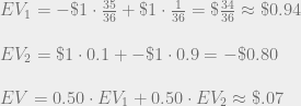
Expected value of saying Heads = 50% chance of Heads $2 gain for saying Heads on both days + 50% chance of Tails $0 = $1

Expected value of saying Tails = 50% chance of Heads $0 + 50% chance of Tails $1 gain for saying Tails on Tuesday = $0.50

So the expected value of saying Heads is still higher even if you think that the probability of Heads and Tails are equal, provided that you know about subjunctive dependence and timeless decision theory!

It’s time for yet another post about the anthropic dice killer thought experiment. 😛

In this post, I’ll point out some features of the thought experiment that have gone unmentioned in this blog thus far. Perhaps it is in these features that we can figure out how to think about this the right way.

First of all, there are lots of hidden infinities in the thought experiment. And as we’ve seen before, where there are infinities, things start getting really wacky. Perhaps some of the strangeness of the puzzle can be chalked up to these infinities.

For instance, we stipulated that the population from which people are being kidnapped is infinite. This was to allow for the game to go on for arbitrarily many rounds, but it leads to some trickiness. As we saw in the last post, it becomes important to calculate the probability of a particular individual being kidnapped if randomly drawn from the population. But… what is this probability if the population is infinite? The probability of selecting a particular person from an infinite population is just like the probability of picking 5 if randomly selecting from all natural numbers: zero!

Things get a little conceptually tricky here. Imagine that you’re randomly selecting a real number between 0 and 1. The probability that you select any particular number is zero. But at the same time, you will end up selecting some number. Whichever number you end up selecting, is a number that you would have said had a 0% chance of being selected! For situations like these, the term “almost never” is used. Rather than saying that any particular number is impossible, you say that it will “almost never” be picked. While this linguistic trick might make you feel less uneasy about the situation, there still seems to be some remaining confusion to be resolved here.

So in the case of our thought experiment, no matter how many rounds the game ends up going on, you have a 0% chance of being kidnapped. At the same time, by stipulation you have been kidnapped. Making sense of this is only the first puzzle. The second one is to figure out if it makes sense to talk about some theories making it more likely than others that you’ll be kidnapped (is smaller than ?)

An even more trouble infinity is in the expected number of people that are kidnapped. No matter how many rounds end up being played, there are always only a finite number of people that are ever kidnapped. But let’s calculate the expected number of people that play the game.

But wait, this sum diverges! To see this, let’s just for a moment consider the expected number of people in the last round:

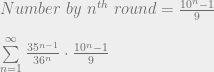
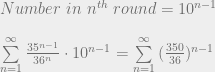
Since , this sum diverges. So on average there are an infinite number of people on the last round (even though the last round always contains a finite number of people). Correspondingly, the expected number of people kidnapped is infinite.

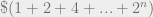
Why might these infinities matter? Well, one reason is that there is a well known problem with playing betting games against sources with infinite resources. Consider the Martingale betting system:

A gambler makes a bet of $1 at some odds. If they win, then good for them! Otherwise, if they lose, they bet $2 on the same odds. If they lose this time, they double down again, betting $4. And so on until eventually they win. The outcome of this is that by the time they win, they have lost and gained . This is a net gain of $1. In other words, no matter what the odds they are betting on, this betting system guarantees a gain of $1 with probability 100%.

However, this guaranteed $1 only applies if the gambler can continue doubling down arbitrarily long. If they have a finite amount of money, then at some point they can no longer double down, and they suffer an enormous loss. For a gambler with finite resources, they stand a very good chance of gaining $1 and a very tiny chance of losing massively. If you calculate the expected gain, it turns out to be no better than what you expect from any ordinary betting system.

Summing up: With finite resources, continually doubling down gives no advantage on average. But with infinite resources, continually doubling down gives a guaranteed profit. Hopefully you see the similarity to the dice killer thought experiment. With an infinite population to draw from, the killer can keep “doubling down” (actually “decupling” down) until they finally get their “payout”: killing all of their current captives. On the other hand, with a finite population, the killer eventually loses the ability to get a new group of 10x the population of the previous one and lets everybody free. In this case, exactly like the Martingale system, the odds for a kidnappee end up coming out to the prior odds of 1/36.

What this indicates is that at least some of the weirdness of the dice killer scenario can be chalked up to the exploitability of infinities by systems like the Martingale system. If you have been kidnapped by the dice killer, you should think that your odds are 90% only if you know you are drawn from an infinite population. Otherwise, your odds should come out to 1/36.

But now consider the following: If you are a casino owner, should you allow into your casino a person with infinite money? Clearly not! It doesn’t matter how much of a bias the games in the casino give in favor of the house. An infinitely wealthy person can always exploit this infinity to give themselves an advantage.

But what about allowing a person with infinite money into your casino to place a single bet? In this case, I think that the answer is yes, you should allow them. After all, with only a finite number of bets, the odds still come out in favor of the house. This is actually analogous to the original dice killer puzzle! You are only selected in one round, and know that you will not be selected at any other time. So perhaps the infinity does not save us here.

One final point. It looks like a lot of the weirdness of this thought experiment is the same type of weirdness as you get from infinitely wealthy people using the Martingale betting system. But now we can ask: Is it possible to construct a variant of the dice killer thought experiment in which the anthropic calculation differs from the non-anthropic calculation, AND the expected number of people kidnapped is finite? It doesn’t seem obvious to me that this is impossible. Since the expected number of captives takes the form of an infinite sum with the number of people by the Nth round multiplied by roughly , all that is required is that the number of people by the Nth round be less than . Then the anthropic calculation should give a different answer from the non-anthropic calculation, and we can place the chance of escape in between these two. Now we have a finite expected number of captives, but a reversal in decision depending on whether you update on anthropic evidence or not. Perhaps I’ll explore this more in future posts.

I recently came up with what I thought was a solution to the dice killer puzzle. It turns out that I was wrong, but in the process of figuring this out I discovered a few subtleties in the puzzle that I had missed first time around.

First I’ll repost the puzzle here:

A mad killer has locked you in a room. You are trapped and alone, with only your knowledge of your situation to help you out.

One piece of information that you have is that you are aware of the maniacal schemes of your captor. His plans began by capturing one random person. He then rolled a pair of dice to determine their fate. If the dice landed snake eyes (both 1), then the captive would be killed. If not, then they would be let free.

But if they are let free, the killer will search for new victims, and this time bring back ten new people and lock them alone in rooms. He will then determine their fate just as before, with a pair of dice. Snake eyes means they die, otherwise they will be let free and he will search for new victims.

His murder spree will continue until the first time he rolls snake eyes. Then he will kill the group that he currently has imprisoned and retire from the serial-killer life.

Now. You become aware of a risky way out of the room you are locked in and to freedom. The chances of surviving this escape route are only 50%. Your choices are thus either (1) to traverse the escape route with a 50% chance of survival or (2) to just wait for the killer to roll his dice, and hope that it doesn’t land snake eyes.

What should you do?

As you’ll recall, there are two possible estimates of the probability of the dice landing snake eyes: 1/36 and 90%. Briefly, the arguments for each are…

Argument 1  The probability of the dice landing snake eyes is 1/36. If the dice land snake eyes, you die. So the probability that you die is 1/36.

Argument 2  The probability that you are in the last round is above 90%. Everybody in the last round dies. So the probability that you die is above 90%.

The puzzle is trying to explain what is wrong with the second argument, given its unintuitive consequences. So, here’s an attempt at a resolution!

Imagine that you find out that you’re in the fourth round with 999 other people. The probability that you’re interested in is the probability that the fourth round is the last round (which is equivalent to the fourth round being the round in which you get snake-eyes and thus die). To calculate this, we want to consider all possible worlds (i.e. all possible number of rounds that the game might go for) and calculate the probability weight for each.

In other words, we want to be able to calculate P(Game ends on the Nth round) for every N. We can calculate this a priori by just considering the conditions for the game ending on the Nth round. This happens if the dice roll something other than snake eyes N-1 times and then snake eyes once, on the final round. Thus the probability should be:

Now, to calculate the probability that the game ends on the fourth round, we just plug in N = 4 and we’re done!

But hold on. There’s an obvious problem with this approach. If you know that you’ve been kidnapped on the fourth round, then you should have zero credence that the game ended on the third, second, or first rounds. But the probability calculation above gives a non-zero credence to each of these scenarios! What’s gone wrong?

Answer: While the probability above is the right prior probability for the game progressing to the Nth round, what we actually want is the posterior probability, conditioned on the information that you have about your own kidnapping.

In other words, we’re not interested in the prior probability P(Game ends on the Nth round). We’re interested in the conditional probability P(Game ends on the Nth round | I was kidnapped in the fourth round). To calculate this requires Bayes’ rule.

The top term P(You are in the fourth round | N total rounds) is zero whenever N is less than four, which is a good sign. But what happens when N is ≥ 4? Does the probability grow with N or shrink?

Intuitively, we might think that if there are a very large number of rounds, then it is very unlikely that we are in the fourth one. Taking into account the 10x growth in number of people each round, it looks like for any N > 4, the theory that there are N rounds strongly predicts that you are in the Nth round. The larger N is, the more strongly it predicts that you are not in the fourth round. In other words, the update on your being in the fourth round strongly favors possible worlds in which the fourth round is the last one

But this is not the whole story! There’s another update to be considered. Remember that in this setup, you exist as a member of a boundless population and are at some point kidnapped. We can ask the question: How likely is it that you would have been kidnapped if there were N rounds?  Clearly, the more rounds there are before the game ends, the more people are kidnapped, and so the higher chance you have of being kidnapped in the first place! This means that we should expect it to be very likely that the fourth round is not the last round, because worlds in which the fourth round is not the last one contain many more people, thus making it more likely that you would have been kidnapped at all.

In other words, we can break our update into two components: (1) that you were kidnapped, and (2) that it was in the fourth round that you were kidnapped. The first of these updates strongly favors theories in which you are not in the last round. The second strongly favors theories in which you are in the last round. Perhaps, if we’re lucky, these two updates cancel out, leaving us with only the prior probability based on the objective chance of the dice rolling snake eyes (1/36)!

Recapping: If we know which round we are in, then when we update on this information, the probability that this round is the last one is just equal to the objective chance that the dice roll lands snake eyes (1/36). Since this should be true no matter what particular round we happen to be in, we should be able to preemptively update on being in the Nth round (for some N) and bring our credence to 1/36.

This is the line of thought that I had a couple of days ago, which I thought pointed the way to a solution to the anthropic dice killer puzzle. But unfortunately… I was wrong. It turns out that even when we consider both of these updates, we still end up with a probability > 90% of being in the last round.

Here’s an intuitive way to think about why this is the case.

In the solution I wrote up in my initial post on the anthropic dice killer thought experiment, I gave the following calculation:

Basically, we look at the fraction of people that die if the game ends on the Nth round, calculate the probability of the game ending on the Nth round, and then average the fraction over all possible N. This gives us the average fraction of people that die in the last round.

We now know that this calculation was wrong. The place where I went wrong was in calculating the chance of getting snake eyes in the nth round. The probability I wrote was the prior probability, where what we want instead is the posterior probability after performing an anthropic update on the fact of your own kidnapping.

So maybe if we plug in the correct values for these probabilities, we’ll end up getting a saner answer!

Unfortunately, no. The fraction of people that die starts at 100% and then gradually decreases, converging at infinity to 90% (the limit of  is .9). This means that no matter what probabilities we plug in there, the average fraction of people will be greater than 90%. (If the possible values of a quantity are all greater than 90%, then the average value of this quantity cannot possibly be less than 90%.)

This means that without even calculating the precise posterior probabilities, we can confidently say that the average probability of death must be greater than 90%. And therefore our proposed solution fails, and the mystery remains.

It’s worth noting that even if our calculation had come out with the conclusion that 1/36 was the actual average chance of death, we would still have a little explaining to do. Namely, it actually is the case that the average person does better by trying to escape (i.e. acting as if the probability of their death is greater than 90%) than by staying around (i.e. acting as if the probability of their death is 1/36).

This is something that we can say with really high confidence: accepting the apparent anthropic calculation of 90% leaves you better off on average than rejecting it. On its own, this is a very powerful argument for accepting 90% as the answer. The rational course of action should not be one that causes us to lose where winning is an option.