The Weirdest Consequence of the Axiom of Choice

This post is about the most startling puzzle I’ve ever heard. First, two warm-up hat puzzles.

Four prisoners, two black hats, two white hats

Four prisoners are in a line, with the front-most one hidden from the rest behind a wall. Each is wearing a hat, but they can’t see its color. There are two black hats and two white hats, and all four know this.

Hat-Puzzle-0-2605645631-1571331493544.png

As soon as any prisoner figures out the color of their own hat, they must announce it. If they’re right, everybody goes free. They cannot talk to each other or look any direction but forwards.

Are they guaranteed freedom?

Solution

Yes, they are! If D sees the same color hat on B and C’s heads, then he can conclude his own hat’s color is the other, so everybody goes free. If he sees differently colored hats, then he cannot conclude his hat color. But C knows this, so if D doesn’t announce his hat color, then C knows that his hat color is different from B’s and they all go free. Done!

Next:

Ten prisoners, unknown number of black and white hats

Hat-Puzzle-927401657-1571331566266.png

Each prisoner is randomly assigned a hat. The number of black and white hats is unknown. Starting from the back, each must guess their hat color. If it matches they’re released, and if not then they’re killed on the spot. They can coordinate beforehand, but cannot exchange information once the process has started.

There is a strategy that gives nine of the prisoners 100% chance of survival, and the other a 50% chance. What is it?

Solution

A10 counts the number of white hats in front of him. If it’s odd, he says ‘white’. Otherwise he says ‘black’. This allows each prisoner to learn their own hat color once they hear the prisoner behind them.

— — —

Alright, now that you’re all warmed up, let’s make things a bit harder.

Countably infinite prisoners, unknown number of black and white hats, no hearing

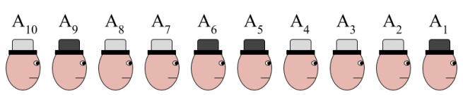
There are a countable infinity of prisoners lined up with randomly assigned hats. They each know their position in line.

Hat-Puzzle-1-3964260265-1571331739116.png

The hat-guessing starts from A1 at the back of the line. Same consequences as before: the reward for a right guess is freedom and the punishment for a wrong guess is death.

The prisoners did have a chance to meet and discuss a plan beforehand, but now are all deaf. Not only can they not coordinate once the guessing begins, but they also have no idea what happened behind them in the line.

The puzzle for you is: Can you find a strategy that ensures that only finitely many prisoners are killed?

Oh boy, the prisoners are in a pretty tough spot here. We’ll give them a hand; let’s allow them logical omniscience and the ability to memorize an uncountable infinity of information. Heck, let’s also give them an oracle to compute any function they like.

Give it a try!

(…)

(…)

Solution

Amazingly, the answer is yes. All but a finite number of prisoners can be saved.

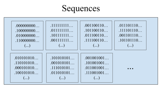
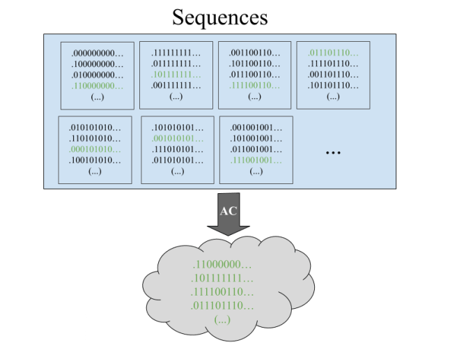
Here’s the strategy. First start out by identifying white hats with the number 0, and black hats with the number 1. Now the set of all possible sequences of hats in the line is the set of all binary sequences. We define an equivalence relation on such sequences as follows: 𝑥 ~ 𝑦 if and only if 𝑥 and 𝑦 are identical after a finite number of digits in the sequence. This will partition all possible sequences into equivalence classes.

Hat Puzzle (2)

For example, the equivalence class of 0 will just be the subset of the rationals whose binary expansion ends at some point (i.e. the subset of the rationals that can be written as an integer over a power of 2). Why? Well, if a binary sequence 𝑥 is equivalent to .000000…, then after a finite number of digits of 𝑥, it will have to be all 0s forever. And this means that it can be written as some integer over a power of 2.

When the prisoners meet up beforehand, they use the axiom of choice to select one representative from each equivalence class. (Quick reminder: the axiom of choice says that for any set 𝑥 of nonempty disjoint sets, you can form a new set that shares exactly one element with each of the sets in 𝑥.) Now each prisoner is holding in their head an uncountable set of sequences, each one of which represents an equivalence class.

Hat Puzzle (3)

Once they’re in the room, every prisoner can see all but a finite number of hats, and therefore they know exactly which equivalence class the sequence of hats belongs to. So each prisoner guesses their hat color as if they were in the representative sequence from the appropriate equivalence class. Since the actual sequence and the representative sequence differ in only finitely many places (all at the start), all entries are going to be the same after some finite number of prisoners. So every single prisoner after this first finite batch will be saved!

laugh-michael-scott

This result is so ridiculous that it actually makes me crack up thinking about it. There is surely some black magic going on here. Remember, each prisoner can see all the hats in front of them, but they know nothing about the total number of hats of each color, so there is no correlation between the hats they see and the hat on their head. And furthermore, they are deaf! So they can’t learn any new information from what’s going on behind them! They literally have no information about the color of their own hat. So the best that each individual could do must be 50/50. Surely, surely, this means that there will be an infinite number of deaths.

But nope! Not if you accept the axiom of choice! You are guaranteed only a finite number of deaths, just a finite number that can be arbitrarily large. How is this not a contradiction? Well, for it to be a contradiction, there has to be some probability distribution over the possible outcomes which says that Pr(finite deaths) = 0. And it turns out that the set of representative sequences form a non-measurable set (a set which cannot have a well-defined size using the ordinary Lebesgue measure). So no probability can be assigned to it (not zero probability, literally undefined)! Now remember that zero deaths occur exactly when the real sequence is one of the representative sequences. This means that no probability can be assigned to this state of affairs. The same thing applies to the state of affairs in which one prisoner dies, or two prisoners, and so on. You literally cannot define a probability distribution over the number of prisoners to die.

By the way, what happens if you have an uncountable infinity of prisoners? Say we make them infinitely thin and then squeeze them along the real line so as to populate every point. Each prisoner can see all but a finite number of the other prisoner’s hats. Let’s even give them hats that have an uncountable number of different colors. Maybe we pick each hat color by just randomly selecting any frequency of visible light.

Turns out that we can still use the axiom of choice to guarantee the survival of all but finitely many prisoners!

colbert-laugh
Colbert’s reaction when he first learned about the uncountable version of the hat problem

One last one.

Countably infinite prisoners, unknown number of black and white hats, with hearing

We have a countable infinity of prisoners again, each with either a black or white hat, but this time they can hear the colors called out by previous prisoners. Now how well can they do?

The answer? (Assuming the axiom of choice) Every single prisoner can be guaranteed to survive except for the first one, who survives with 50% probability. I really want this to sink in. When we had ten prisoners with ten hats, they could pull this off by using their knowledge of the total number of black and white hats amongst them. Our prisoners don’t have this anymore! They start off knowing nothing about the number of white and black hats besides what they can see in front of them. And yet they still get out of it with all but one prisoner guaranteed freedom.

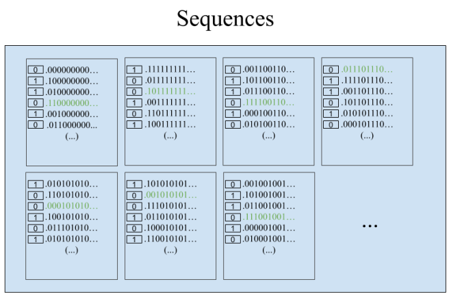
How do they do this? They start off same as before, defining the equivalence relation and selecting a representative sequence from each equivalence class. Now they label every single sequence with either a 0 or a 1. A sequence gets a 0 if it differs from the representative sequence in its equivalence class in an even number of places, and otherwise it gets a 1. This labeling has the result that any two sequences that differ by exactly one digit have opposite labels.

Hat-Puzzle-4.png

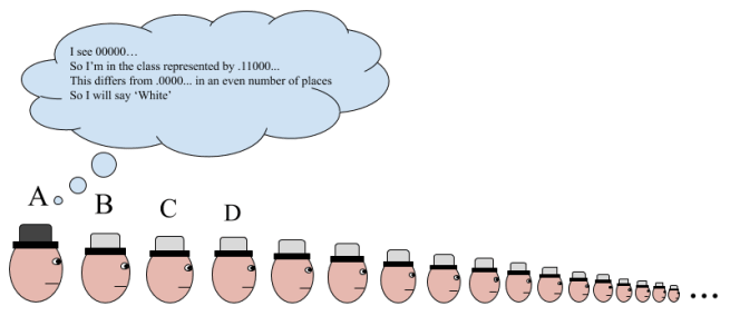
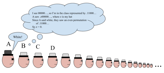
Now the first person (A) just says the label of the sequence he sees. For the next person up (B), this is the sequence that starts with their hat. And remember, they know which equivalence class they’re in, since they can see everybody in front of them! So all they need to do is consider what the label of the sequence starting with them would be if they had a white hat on. If it would be different than the label they just heard, then they know that their hat is black. And if it would be the same, then their hat is white!

The person in front of B knows the equivalence class they’re in, and now also knows what color B’s hat was. So they can do the exact same reasoning to figure out their hat color! And so on, saving every last countable prisoner besides A..

Let’s see an example of this, for the sequence 100000…

Hat-Puzzle-5.png

Hat Puzzle (6)

Hat Puzzle (7)Hat-Puzzle-8.png

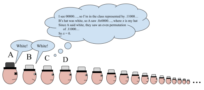
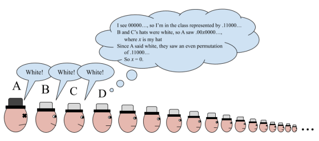
And so on forever, until every last prisoner besides A is free.

This set of results is collectively the most compelling argument I know for rejecting AC, and I love it.

Introduction to Mathematical Logic (Part 3: Reconciling Gödel’s Completeness And Incompleteness Theorems)

Last time we saw that no first-order theory could successfully pin down the natural numbers as a unique model. We also saw that in fact no sound and complete theory with the property of finite provability could pick out ℕ; any such theory has a Compactness Theorem, from which you can prove the existence of nonstandard models of numbers that include infinities of numbers larger than any of the naturals.

Worse, we saw that due to the Löwenheim-Skolem theorem, any first-order theory of the naturals has uncountable models, as well as models of every infinite cardinality. What followed from this was that try as we might, any first-order theory will fail to prove elementary facts about the natural numbers, like that there are a countable infinity of them or that no number is larger than 0, 1, 2, 3, and all the rest of the standard naturals.

Now, with the limitations in our ability to prove all true facts about the natural numbers firmly established, I want to talk about a theorem that seems to be in contradiction with this. This is the Completeness Theorem, proven by the same Kurt Gödel who later discovered the Incompleteness Theorems.

In a few words, the Completeness Theorem says that in any first-order theory, that which is semantically entailed is also syntactically entailed. Or, said differently, the Completeness Theorem says that a first order theory can prove everything that is true in all its models.

This sounds great! It’s the dream of mathematicians to be able to construct a framework in which all truths are provable, and Gödel appears to be telling us that first order logic is just such a framework.

But hold on, how do we reconcile this with what we just said: that there are true facts about the natural numbers that can’t be proven? And how do we reconcile this with what Gödel later proved: the Incompleteness Theorems? The First Incompleteness Theorem shows that that in any axiomatic system of mathematics, there will be true statements about arithmetic that cannot be proven within the system. These seem to be in stark contradiction, right? So which is right; Completeness or Incompleteness? Can we prove everything in first-order logic or not?

It turns out that there is no contradiction here. The Completeness Theorem is true of first order logic, as is the Incompleteness Theorem. What’s required is a subtle understanding of exactly what each theorem is saying to understand why the apparent conflict is only apparent.

There are two senses of completeness. One sense of completeness refers to theories in a particular logic. In this sense, a theory is complete if it can prove the truth or falsity of every well-formed formula. Gödel’s Incompleteness Theorems are about this sense of completeness: no theory rich enough to talk about the natural numbers can prove all statements about the natural numbers.

The second sense of completeness refers to logical frameworks themselves. A logical framework is complete if for every theory in that logic, all the semantically valid statements can be proven. Gödel’s Completeness Theorem is about this sense of completeness. In first-order logic, any theory’s semantic consequences are syntactic consequences.

Let’s go a little deeper into this.

What Gödel showed in his First Incompleteness Theorem is that one can encode the statements of any logical theory (first order or second order) as natural numbers. Then, if your theory is expressive enough to talk about the natural numbers, you produce a type of circularity: Your theory makes statements about the natural numbers, and the natural numbers encode statements from the theory. Gödel exploited this circularity to produce a sentence whose interpretation is something like “This sentence has no proof in T” (where T is your chosen theory). This sentence corresponds to some complicated fact about the properties of the natural numbers, because all sentences are encoded as natural numbers. If it’s false, then that means that the sentence does have a proof, so it’s true. And if it’s true, then it has no proof. The conclusion is that for any theory T, there are true statements about the natural numbers that cannot be proven by T.

The Incompleteness Theorem plays out slightly differently in first and second order logic. In first-order logic, anything that’s true in all models is provable. It’s just that there is no theory that has the natural numbers as a unique model. The best you can do in first-order logic is develop a theory that has the natural numbers as one out of many models. But this means that there is no first-order theory whose semantic consequences are all the truths about the natural numbers! (This is a neat way to actually prove the inevitability of nonstandard models of arithmetic, as a necessary consequence of the combination of the Completeness and Incompleteness theorems.)

And as it happens, any theory that has a model of the natural numbers is also going to have models in which Gödel’s statement is actually false! Remember that Gödel’s statement, if false, says that it is provable, which is to say that some number encodes a proof of it. In nonstandard models of arithmetic, there will be nonstandard numbers that encode a “proof” of Gödel’s statement, using Gödel’s encoding. It’s just that these “proofs” are not actually going to be things that we recognize as valid (for example, nonstandard numbers can represent infinitely long proofs). They’re proofs according to Gödel’s encoding, but Gödel’s encoding only represents valid proofs insofar as we assume that only natural numbers are being used in the encoding. So since Gödel’s statement is not true in all models of any first-order theory of arithmetic, it’s not provable from the axioms of the theory. And this is totally consistent with any first-order theory being complete! All that completeness means is that anything that is true in all models of a theory is also provable!

Now, how does this play out in second-order logic? Well, in second-order logic, you can uniquely pin down the natural numbers with a second-order theory. This is where the Incompleteness Theorem swoops in and tells you that the semantic consequences are not all syntactic consequences. Since there are second-order theories whose semantic consequences are all the truths about the natural numbers, these theories must have as semantic consequences the truth of the Gödel statement, which by construction means that they cannot have the Gödel statement as a syntactic consequence.

So either way you go, first or second order, you’re kinda screwed. In first-order, you can prove all the semantic consequences of a theory. It’s just that no theory has the full set of semantic consequences that we want, because first-order logic doesn’t have the expressive power to pin down the types of mathematical structures that we are interested in. And in second-order theories, you do have the expressive power to pin down the types of mathematical structures we care about, but as a consequence lose the property that all semantic consequences can be proved.

Regardless, there are fundamental limitations in our ability to prove all the facts that we want to prove as mathematicians. Hilbert’s program has crumbled. You can choose a theory that guarantees you the ability to prove all its semantic consequences, but lacks the expressive power to uniquely pin down the natural numbers. Or you can choose a theory that has the expressive power to uniquely pin down the natural numbers, but guarantees you the inability to prove all its semantic consequences.

Introduction to Mathematical Logic (Part 2: The Natural Numbers)

Previously, we talked about the distinction between a logic, a language, a theory, and a model, and introduced propositional and first order logic. We toyed around with some simple first-order models, and began to bump our heads against the expressive limitations of the language of first order logic. Now it’s time to apply what we’ve learned to some REAL math! Let’s try to construct a first order theory of the natural numbers. N = {0, 1, 2, 3, …}

The first question we have to ask ourselves is what our language should be. What constants, predicates, and functions do we want to import into first order logic? There are many ways you could go here, but one historically popular approach is the following:

Constants: 0
Functions: S, +, ×
Predicates: ≥

We add just one constant, 0, three functions (a successor function to get the rest of the numbers from 0, as well as addition and multiplication), and one predicate for ordering the numbers. Let’s actually make this a little simpler, and talk about a more minimal language for talking about numbers:

Constants: 0
Functions: S
Predicates: None

This will be a good starting point, and from here we can easily define +, ×, and ≥ if necessary later on. Now, take a look at the following two axioms:

  1. x (Sx ≠ 0)
  2. xy (x ≠ y → Sx ≠ Sy)

In plain English, axiom 1 says that 0 is not the successor of any number. And axiom 2 says that two different numbers can’t have the same successor.

Visually, the first axiom tells us that this situation can’t happen:

Untitled document (1)

And the second axiom tells us that this situation can’t happen:

Untitled-document-2.png

Now, we know that 0 is a number, because it’s a constant in our language.

Untitled document

By axiom 1, we know that S0 cannot be 0. So it’s something new.

Untitled document (3)

S0 cannot go to 0, because of axiom 1. And it can’t go to itself, as that would be a violation of axiom 2. So it has to go to something new:

Untitled document (4)

Now, where does SS0 get sent? Not to 0, for the same reason as before. And not to either S0 or SS0, because then we’d have a violation of axiom 2. So it must go to a new number. You can see where this is going.

Untitled document (5)

These two axioms really cleverly force us to admit an infinite chain of unique new numbers. So is that it? Have we uniquely pinned down the natural numbers?

It turns out that the answer is no. Consider the following model:

Untitled document (6)

This is perfectly consistent with our axioms! No number goes to 0 via the successor function, and no two different numbers have the same successor. But clearly this is not a model of the natural numbers. One quick and easy patch on this is just to add a new axiom, banning any numbers that are their own successor.

3. ∀x (Sx ≠ x)

Now, we’ve taken care of this problem, but it’s a symptom of a larger issue. Here’s a model that’s perfectly consistent with our new axioms:

Untitled document (7)

In the same vein as before, we can patch this with a new axiom, call it 3’:

3’. x (SSx ≠ x)

But now we have the problem of three-loops, which require their own axiom to be ruled out (3’’. x (SSSx ≠ x)). And in general, this approach will end up requiring us to have an infinite axiom schema, one axiom for each loop length that we need to ban.

However, even then we’re not done! Why? Well, once we’ve banned all loops, we run into the following problem:

Untitled document (8)

We can fix this by specifying that 0 is the only number that is not the successor of any number. Formally, this looks like:

x (y (Sy ≠ x) → x = 0)

Okay, so that takes care of other copies of the natural numbers. But we’re still not done! Take a look at the following model:

Untitled document (9)

This model violates none of our axioms, but is clearly not the natural numbers. We’re running into a lot of problems here, and our list of axioms is getting really long and unwieldy. Is there any simpler system of axioms that will uniquely pin down the natural numbers for us?

The amazing fact is that no, this is not possible. In fact, no matter how hard you try, you will never be able to rule out models of your axioms that contain “nonstandard numbers” in first-order logic.

We’ll prove this using a beautiful line of reasoning, which I think of as one of the simplest and most profound arguments I’ve encountered. There’s several subtle steps here, so read carefully:

Step 1

We’re going to start out by proving a hugely important theorem called the Compactness Theorem.

  • Suppose that a first order theory T has no model.
  • Then there is no consistent assignment of truth values to all WFFs.
  • So you can prove a contradiction from T. (follows from completeness)
  • All proofs must be finite, so if you can prove a contradiction from T, you can do it in a finite number of steps.
  • If the proof of contradiction takes a finite number of steps, then it uses only a finite number of T’s axioms.
  • So there is a proof of contradiction from a finite subset of T’s axioms.
  • So there’s a finite subset of T’s axioms that has no model. (follows from soundness)
  • So if T has no model, then there’s a finite subset of T’s axioms that has no model.

The Compactness Theorem as it’s usually stated is the contrapositive of this: If all finite subsets of T’s axioms have a model, then T has a model. If you stop to think about this for a minute, it should seem pretty surprising to you. (It’s trivial for the case that T contains a finite number of axioms, of course, but not if T has an infinity of axioms.)

Also notice that our proof of the theorem barely relied on what we’ve said about the properties of first order logic at all! In fact, it turns out that there is a Compactness Theorem in any logic that is sound (syntactic entailment implies semantic entailment, or in other words: that which is provable is true in all models), complete (semantic entailment implies syntactic entailment, or: that which is true in all models is provable), and only allows finite proofs.

In other words, any logic in which the provable statements are exactly those statements that are true in all models, no more and no less, and in which infinite proofs are considered invalid, will have this peculiar property.

Step 2

Now, we use the Compactness Theorem to prove our desired result.

  • Suppose we have a first order theory T that has the natural numbers N as a model.
  • We create a new theory T’ by adding a constant symbol ω and adjoining an infinite axiom schema:
    • ‘ω ≥ 0’
    • ‘ω ≥ S0’
    • ‘ω ≥ SS0’
    • ‘ω ≥ SSS0’ (And so on…)
  • N is no longer a model of T’, because T’ says that there is a number that’s larger than every natural number, which is false in N.
  • But T’ still has a model, because of compactness:
    • Any finite subset of the axioms of T’ has a finite number of statements that look like ‘ω > x’. But this is consistent with ω being a natural number! (because for any set of natural numbers you can find a larger natural number)
    • So N is a model of any finite subset of the axioms of T’.
    • So by compactness, T’ has a model. This model is nonstandard (because earlier we saw that it’s not N).
  • Furthermore, any model of T’ is a model of T, because T’ is just T + some constraints.
  • So since T’ has a nonstandard model, so does T.
  • Done!

The conclusion is the following: Any attempt to model N with a first order theory is also going to produce perverse nonstandard models in which there are numbers larger than any natural number.

Furthermore, this implies that no first order theory of arithmetic can prove that there is no number larger than every natural number. If we could, then we would be able to rule out nonstandard models. But we just saw that we can’t! And in fact, we can realize that ω, as a number, must have a successor, which can’t be itself, and which will also have a successor, and so on forever, so that we will actually end up with an infinity of infinitely-large numbers, none of which we have any power to deny the existence of.

But wait, it gets worse! Compactness followed from just three super elementary desirable features of our logic: soundness, completeness, and finite provability. So this tells us that our inability to uniquely pin down the natural numbers is not just a problem with first order logic, it’s basically a problem with any form of logic that does what we want it to do.

Want to talk about the natural numbers in a Hilbertian logical framework, where anything that’s true is provable and anything that’s provable is true? You simply cannot. Anything you say about them has to be consistent with an interpretation of your statements in which you’re talking about a universe with an infinity of infinitely large numbers.

Löwenheim-Skolem Theorem

Just in case your mind isn’t sufficiently blown by the Compactness Theorem and its implications, here’s a little bit more weirdness.

The Löwenheim-Skolem Theorem says the following: If a first-order theory has at least one model of any infinite cardinality, then it has at least one model of EVERY infinite cardinality.

Here’s an intuition for why this is true: Take any first order theory T. Construct a new theory T’ from it by adding κ many new constant symbols to its language, for any infinite cardinality κ of your choice. Add as axioms c ≠ c’, for any two distinct new constant symbols. The consistency of the resulting theory follows from the Compactness Theorem, and since we got T’ by adding constraints to T, any model of T’ must be a model of T as well. So T has models of any infinite cardinality!

The Löwenheim-Skolem Theorem tells us that any first order theory with the natural numbers as a model also has models the size of the real numbers, as well as models the size of the power set of the reals, and the power set of the power set of the reals, and so on forever. Not only can’t we pin down the natural numbers, we can’t even pin down their cardinality!

And in fact, we see from this that no first-order statement can express the property of “being a specific infinite cardinality.” If we could do this, then we could just add this statement to a theory as an axiom and rule out all but one infinite cardinality.

Here’s one more for you: The Löwenhiem-Skolem Theorem tells us that any attempt to talk about the real numbers in first order logic will inevitably have an interpretation that refers solely to a set that contains a countable infinity of objects. This implies that in first order logic, almost all real numbers cannot be referred to!

Similarly, a first order set theory must have countable models. But keep in mind that Cantor showed how we can prove the existence of uncountably infinite sets from the existence of countably infinite sets! (Namely, just take a set that’s countably large, and power-set it.) So apparently, any first order set theory has countable models that… talk about uncountable infinities of sets? This apparent contradiction is known as Skolem’s paradox, and resolving it leads us into a whole new set of strange results for how to understand the expressive limitations of first order logic in the context of set theory.

All that and more in a later post!

Introduction to Mathematical Logic (Part 1)

Mathematical logic is the study of the type of reasoning we perform when we do mathematics, and the attempt to formulate a general language as the setting in which all mathematics is done. In essence, it is an attempt to form a branch of mathematics, of which all other branches of mathematics will emerge as special cases.

You might sort of think that when speaking at this level of abstraction, there will nothing general and interesting to say. After all, we’re trying to prove statements not within a particular domain of mathematics, but theorems that are true across a wide swath of mathematics, potentially encompassing all of it.

The surprising and amazing thing is that this is not the case. It turns out that there are VERY general and VERY surprising things you can discover by looking at the logical language of mathematics, a host of results going by names like the Completeness Theorem, the Incompleteness Theorem, the Compactness Theorem, the Löwenheim-Skolem Theorem, and so on. These results inevitably have a great deal of import to our attitudes towards the foundations of mathematics, being that they generally establish limitations or demonstrate eccentricities in the types of things that we can say in the language of mathematics.

My goal in this post is to provide a soft introduction to the art of dealing in mathematics at this level of ultimate abstraction, and then to present some of the most strange things that we know to be true. I think that this is a subject that’s sorely missing this type of soft introduction, and hope I can convey some of the subject’s awesomeness!

— — —

To start out with, why think that there is any subject matter to be explored here? Different branches of mathematics sometimes appear to be studying completely different types of structures. I remember an anecdote from an old math professor of mine, who worked within one very narrow and precisely defined area of number theory, and who told me that when she goes to talks that step even slightly outside her area of specialty, the content of the  lectures quickly incomprehensible to her. Why think that there is such a common language of mathematics, if specialists in mathematics can’t even understand each other when talking between fields?

The key thing to notice here is that although different fields of mathematics are certainly wildly different in many ways, there nevertheless remain certain fundamental features that are shared in all fields. Group theorists, geometrists, and number theorists will all accept the logical inference rule of modus ponens (if P is true and P implies Q, then Q is true), but none of them will accept its converse (if Q is true and P implies Q, then P is true). No matter what area of mathematics you study, you will accept that if P(x) is true for all x, then it is true for any particular x you choose. And so on. These similarities may seem obvious and trivial, but they HAVE to be obvious and trivial to be things that every mathematician agrees on. The goal, then, is to formalize a language that has these fundamental inference rules and concepts built in, and that has many special cases to account for the differences between domains of math, specified by some parameters that are freely chosen by any user of the system.

There are actually several distinct systems that attempt to accomplish this task. Generally speaking, there are three main branches, in order of increasing expressive power: propositional logic, first order (predicate) logic, and second order logic.

Reasoning In Zeroth Order

Let’s start with propositional logic, sometimes called “zeroth order logic.” Propositional logic is the framework developed to deal with the validity of the following types of arguments:

Argument 1

  1. 2+2=4.
  2. If 2+2=4, then 1+3=4.
  3. So 1+3=4.

Argument 2

  1. The Riemann hypothesis is false and P = NP.
  2. So P = NP.

Notice that it doesn’t matter if our premises are true or not. Logical validity doesn’t care about this, it just cares that the conclusions really do follow from the premises. This is a sign of the great generality at which we’re speaking. We’re perfectly fine with talking about a mathematical system in which the Riemann hypothesis is false, or in which 2+2 is not 4, just so long as we accept the logical implications of our assumptions.

Propositional logic can express the validity of these arguments by formalizing rules about valid uses of the concepts ‘and’, ‘if…then…’, ‘or’, and so on. It remains agnostic to the subject matter being discussed by not fully specifying the types of sentences that are allowed to be used in the language. Instead, any particular user of the language can choose their set of propositions that they want to speak about.

To flesh this out more, propositional logic fulfills the following three roles:

  1. Defines an alphabet of symbols.
  2. Specifies a set of rules for which strings are grammatical and which are not.
  3. Details rules for how to infer new strings from existing strings.

In more detail:

  1. The set of symbols in propositional logic are split into two categories: logical symbols and what I’ll call “fill-in-the-blank” symbols. The logical symbols are (, ), , , ¬, and →. The fill-in-the-blank symbols represent specific propositions, that are specified by any particular user of the logic.
  2. Some strings are sensible and others not. For example, the string “P∧∧” will be considered to be nonsensical, while “PQ” will not. Some synonyms for sensible strings are well-formed formulas (WFFs), grammatical sentences, and truth-apt sentences. There is a nice way to inductively generate the set of all WFFs: Any proposition is a WFF, and for any two WFFs F and F’, the following are also WFFs: (FF’), (FF’), ¬F, (F→F’).
  3. These include rules like modus ponens (from P and P→Q, derive Q), conjunction elimination (from PQ, derive P), double negation elimination (from ¬¬P, derive P), and several more. They are mechanical rules that tell you how to start with one set of strings and generate new ones in a logically valid way, such that if the starting strings are true than the derived ones must also be true. There are several different but equivalent formulations of the rules of inference in propositional logic.

A propositional language fills in the blanks in the logic. Say that I want to talk about two sentences using propositional logic: “The alarm is going off”, “A robber has broken in.” For conciseness, we’ll abbreviate these two propositions as A for alarm and R for robber. All I’ll do to specify my language is to say “I have two propositions: {A, R}”

The next step is to fill in some of the details about the relationships between the propositions in my language. This is done by supplementing the language with a set of axioms, and we call the resulting constrained structure a propositional theory. For instance, in my example above we might add the following axioms:

  1. A→R
  2. AR

In plain English, these axioms tell us that (1) if the alarm is going off, then a robber has broken in, and (2) an alarm is going off or a robber has broken in.

Finally, we talk about the models of our theory. Notice that up until now, we haven’t talked at all about whether any statements are true or false, just about syntactic properties like “The string P¬ is not grammatical” and about what strings follow from each other. Now we interpret our theory by seeing what possible assignments of truth values to the WFFs in our language are consistent with our axioms and logical inference rules. In our above example, there are exactly two interpretations:

Model 1: A is true, R is true
Model 2: A is false, R is true

These models can be thought of as the possible worlds that are consistent with our axioms. In one of them, the alarm has gone off and a robber has broken in, and in the other, the alarm hasn’t gone off and the robber has broken in.

Notice that R turns out true in both models. When a formula F is true in all models of a theory, we say that the theory semantically entails F, and write this as T F. When a formula can be proven from the axioms of the theory using the rules of inference given by the logic, then we say that the theory syntactically entails F, and write this as T F.

This distinction between syntax and semantics is really important, and will come back to us in later discussion of several important theorems (notably the completeness and incompleteness theorems). To give a sneak peek: above we found that R was semantically entailed by our theory. If you’re a little familiar with propositional logic, you might have also realized that R can be proven from the axioms. In general, syntactic truths will always be semantic truths (if you can prove something, then it must be true in all models, or else the models would be inconsistent. But a model is by definition a consistent assignment of truth values to all WFFs). But a natural question is: are all semantic consequences of a theory also syntactic consequences? That is, are all universal truths of the theory (things that are true in every model of the theory) provable from the theory?

Summary of mathematical logic meeting

If the answer is yes, then we say that our logic is complete. And it turns out that the answer is yes, for propositional logic. Whether more complex logics are complete turns out to be a more interesting question. More on this later.

This four-step process I just laid out (logic to language to theory to model) is a general pattern we’ll see over and over again. In general, we have the following division of labor between the four concepts:

  1. Logic: The logic tells us the symbols we may use (including some fill-in-the-blank categories of symbols), the rules of grammar, and a set of inference rules for deriving new strings from an existing set.
  2. Language: The language fills in the blanks in our logic, fully specifying the set of symbols we will be using.
  3. Theory: The theory adds axioms to the language.
  4. Model: A model is an assignment of truth values to all WFFs in the language, consistent with the axioms and the inference rules of our logic.

It’s about time that we apply this four-step division to a more powerful logic. Propositional logic is pretty weak. Not much interesting math can be done in a purely propositional language, and it’s wildly insufficient to capture our notion of logically valid reasoning. Consider, for example, the following argument:

  1. Socrates is a man.
  2. All men are mortal.
  3. So, Socrates is mortal.

This is definitely a valid argument. No rational agent could agree that 1 and 2 are true, and yet deny the truth of 3. But can we represent the validity of this argument in propositional logic? No!

Consider that the three sentences “Socrates is a man”, “All men are mortal”, and “Socrates is mortal” are distinct propositions, and the relationships between them are too subtle for propositional logic to capture. Propositional logic can’t see that the first proposition is asserting the membership of Socrates to a general class of things (“men”), and that the second proposition is then making a statement about a universal property of things in this class. It just sees two distinct propositions. To propositional logic, this argument just looks like

  1. P
  2. Q
  3. Therefore, R

But this is not logically valid! We could make it valid by adding as a premise the sentence (PQ)→R, which corresponds to the English sentence “If Socrates is a man and all men are mortal, then Socrates is mortal.” But this should be seen as a tautology, something that is provable in any first order theory that contains the propositions P Q and R, not a required additional assumption. Worse, if somebody came along and stated the proposition A = “Aristotle is a man”, then we would need a whole ‘nother assumption to assert that Aristotle is also mortal! And in general, for any individual instance of this argument, we’d need an independent explanation for its validity. This is not parsimonious, and indicative that propositional logic is missing something big.

Missing what? To understand why this argument is valid, you must be able to reason about objects, properties, and quantification. This is why we must move on to an enormously more powerful and interesting logic: first order logic.

Reasoning In First Order

First order logic is a logic, so it must fill the same three roles as we saw propositional logic did above. Namely, it must define the alphabet, the grammar, and the inference rules.

Symbols
Logical: ¬ → ( ) =
Variables: x y z w …
Constants: ______
Predicates: ______
Functions: ______

That’s right, in first order we have three distinct categories of fill-in-the-blank symbols. Intuitively, constants will be names that refer to objects, predicates will be functions from objects to truth values, and functions will take objects to objects. To take an everyday example, if the objects in consideration are people, then we might take ‘a’ to be a constant referring to a person named Alex, ’T’ to be a predicate representing ‘is tall’, and ‘f’ to be a function representing “the father of”. So T(a) is either true or false, while f(a) doesn’t have a truth value (it just refers to another object). But T(f(a)) does have a truth value, because it represents the sentence “Alex’s father is tall.”

Next, we define well-formed formulas. This process is more complicated than it was for propositional logic, because we have more types of things than we did before, but it’s not too bad. We start by defining a “term”. The set of terms is inductively generated by the following scheme: All constants and variables are terms, and any function of terms is itself a term. Intuitively, the set of terms is the set of objects that our language is able to “point at”.

With the concept of terms in hand, we can define WFFs through a similar inductive scheme: Any predicate of terms is a WFF. And for any WFFs F and F’, (FF’), (FF’), (¬F), (F→F’), x F, x F are all WFFs. The details of this construction are not actually that important, I just think it’s nice how you can generate all valid first order formulas from fairly simple rules.

Good! We have an alphabet, a grammar, and now all we need from our logic is a set of inference rules. It turns out that this set is just going to be the inference rules from propositional logic, plus some new ones:

Quantifier elimination: From x P(x) derive P(t) (for any term t and predicate P)
Quantifier introduction: From P(t) derive x P(x) (for any term t and predicate P)

That’s it, we’ve defined first order logic! Now let’s talk about a first order language. Just like before, the language is just obtained by filling in the blanks left open by our logic. So for instance, we might choose the following language:

Constants: a
Functions: f
Predicates: none

In specifying our function, we have to say exactly what type of function it is. Functions can take as inputs a single object (“the father of”) or multiple objects (“the nearest common ancestor of”), and this will make a difference to how they are treated. So for simplicity, let’s say that our function f just takes in a single object.

A first order theory will simply be a language equipped with some set of axioms. Using our language above, we might have as axioms:

  1. x (f(x) ≠ x)
  2. x (f(x) ≠ a)

In plain English, we’re saying that f never takes any object to itself or to a.

And lastly, we get to the models of a first order theory. There’s an interesting difference between models here and models in propositional logic, which is that to specify a first order model, you need to first decide on the size of your set of objects (the size of the ‘universe’, as it’s usually called), and then find a consistent assignment of truth values to all propositions about objects in this universe.

So, for instance, we can start searching for models of our theory above by starting with models with one object, then two objects, then three, and so on. We’ll draw little diagrams below in which points represent objects, and the arrow represents the action of the function f on an object.

  1. No 1-element universe.
    Summary-of-mathematical-logic-meeting-1.png
  2. No 2-element universe.
    Summary-of-mathematical-logic-meeting-2.png
  3. 3-element universe
    Summary-of-mathematical-logic-meeting-3.png
  4. 4 element universes
    Summary-of-mathematical-logic-meeting-5.pngSummary-of-mathematical-logic-meeting-4.pngSummary-of-mathematical-logic-meeting-7.pngSummary of mathematical logic meeting (6)
  5. And so on…

It’s a fun little exercise to go through these cases and see if you can figure out why there are no models of size 1 or 2, or why the one above is the only model of size 3. Notice, by the way, that in the last two images, we have an object for which there is no explicit term! We can’t get there just using our constant and our functions. Of course, in this case we can still be clever with our quantifiers to talk about the Nameless One indirectly (for instance, in both of these models we can refer to the object that is not equal to a, f(a), or f(f(a))) But in general, the set of all things in the universe is not going to be the same as the set of things in the universe that we can name.

Here’s a puzzle for you: Can you make a first order sentence that says “I have exactly four objects”? That is, can you craft a sentence that, if added as an axiom to our theory, will rule out all models besides the ones that have exactly four elements?

(…)

(Think about it for a moment before moving on…)

(…)

Here’s how to do it for a universe with two objects (as well as a few other statements of interest). The case of four objects follows pretty quickly from this.

  • “I have at most two objects” = xyz (z=x z=y)
  • “I have exactly two objects” = xy (x≠y z(z=x z=y))
  • “I have at least two objects” = xy (x≠y)

Another puzzle: How would you say “I have an infinity of objects”, ruling out all finite models?

(…)

(Think about it for a moment before moving on…)

(…)

This one is trickier. One way to do it is to introduce an infinite axiom schema: “I have at least n objects” for each n.

This brings up an interesting point: theories with infinite axioms are perfectly permissible for us. This is a choice that we make that we could perfectly well deny, and end up with a different and weaker system of logic. How about infinitely long sentences? Are those allowed? No, not in any of the logics we’re talking about here. A logic in which infinite sentences are allowed is called an infinitary logic, and I don’t know too much about such systems (besides that propositional, first, and second order logics are not infinitary).

Okay… so how about infinitely long derivations? Are those allowed? No, we won’t allow those either. This one is more easy to justify, because if infinite derivations were allowed, then we could prove any statement P simply by the following argument “P, because P, because P, because P, because …”. Each step logically follows from the previous, and in any finite system we’d eventually bottom out and realize that the proof has no basis, but in a naive infinite-proof system, we couldn’t see this.

Alright, one last puzzle. How would you form the sentence “I have a finite number of objects”? I.e., suppose you want to rule out all infinite models but keep the finite ones. How can you do it?

(…)

(Think about it for a moment before moving on…)

(…)

This one is especially tricky, because it turns out to be impossible! (Sorry about that.) You can prove, and we will prove in a little bit, that no first order axiom (or even infinite axiom schema) is in general capable of restricting us to finite models. We have run up against our first interesting expressive limitation of first-order logic!

Okay, let’s now revisit the question of completeness that I brought up earlier. Remember, a logic is complete if for any theory in that logic, the theory’s semantic implications are the same as its syntactic implications (all necessary truths are provable). Do you think that first order logic is complete?

The answer: Yes! Kurt Gödel proved that it is in his 1929 doctoral dissertation. Anything that is true in all models of a first order theory, can be proven from the axioms of that theory (and vice versa). This is a really nice feature to have in a logic. It’s exactly the type of thing that David Hilbert was hoping would be true of mathematics in general. (“We must know. We will know!”) But this hope was dashed by the same Kurt Gödel as above, in his infamous incompleteness theorems.

There will be a lot more to say about that in the future, but I’ll stop this post for now. Next time, we’ll harness the power of first order logic to create a first order model of number theory! This will give us a chance to apply some powerful results in mathematical logic, and to discover surprising truths about the logic’s limitations.

Thinking in first order: Are the natural numbers countable?

Here’s a weird fact about first-order logic: there is no first-order theory that has as a model the natural numbers and only the natural numbers. Any first-order theory talking about N can only say things that are also consistent with weird other systems that include uncountable infinities of nonstandard numbers. Here’s the proof:

Take first order Peano arithmetic (PA). We know that the natural numbers N are a model of PA, because all the axioms are true of PA. Now add a constant c to your language, and adjoin an infinite axiom schema: ‘c > 0’, ‘c > S0’, ‘c > SS0’, and so on. Call this new theory PA(c).

The natural numbers are clearly no longer a model of PA(c), because PA(c) says that there’s a number that’s larger than all natural numbers, which is false in N. But we can prove that PA(c) still has a model! We prove this using the Compactness Theorem, which tells us that a theory has a model if every finite subset of its axioms has a model. Consider any finite subset of the axioms of PA(c). For any such subset, there are only finitely many statements that look like c > X. So there are only finitely many numbers that c is larger than. But then this is always going to be satisfied by N! For any collection of natural numbers, you can always find a natural number larger than all of then. So N is a model of every finite subset of the axioms of PA(c). But then, by compactness, since every finite subset of the axioms of PA(c) has a model, PA(c) has a model!

Final step in the proof: PA(c) has a model, and this model is definitely not the natural numbers. Call it a nonstandard model. But now note that PA(c) was obtained from PA just by adding axioms. Adding axioms never increases the number of models, it only narrows them down. So if the nonstandard model is a model of PA(c), then it also must be a model of PA! And there it is, we’ve proved that first order Peano arithmetic has more models than the natural numbers.

Notice, also, that it didn’t matter that we started with first order Peano arithmetic. We could have started with any first order theory that has N as a model, added the constant c, and adjoined on the infinite axiom schema corresponding to c being larger than all natural numbers! So what we’ve actually proven is that no first order theory can “pin down” the natural numbers. Any first order theory that has N as a model, also has weird extra models that allow numbers greater than all natural numbers. Furthermore, you can then run the exact same type of proof again, adjoining a new constant that’s larger than all natural numbers and also larger than c, and by compactness show that it has a model, so that you’ve now found that any first order theory that has N as a model also has a model that has the natural numbers, plus a number larger than all natural numbers, plus a number that’s larger than even that. And you can do this an uncountable infinity of times, and end up proving that if your favored theory has N as a model, then it also has a model whose size is an uncountable infinity. And in fact, any first order theory that has N as a model, also has models of every infinite cardinality.

This is super wild, and really important. Why does it matter that we can’t pin down the natural numbers using any first order theory? Well, think about the set of statements that are true of N, but false of these nonstandard models. These include “there is no number larger than all natural numbers” and “There are a countable infinity of natural numbers”. These statements are not true in all models of any first order theory of N. And if they’re false in some models, then they can’t be proven from the axioms of the theory! (If the theory could prove a statement that was false in one of its models, then the model wouldn’t have been a model of the theory in the first place; models are consistent assignments of truth values to the sentences of the theory.)

In other words, no first order theory of the natural numbers can prove that the natural numbers are countable, or that no number is greater than all natural numbers. If you were a being that could only think in first-order sentences, then you would be unable to conclude these basic facts. To say these things, you need to go up a level to second-order logic, and quantify over properties in addition to objects. Even weirder, if you could only think in first-order logic, you wouldn’t even be able to talk about the natural numbers. No matter how hard you tried to say what you meant by the natural numbers, you would always fail to pin down just the natural numbers. There’d always be room for ambiguity, and everything you said and thought could be equally well interpreted as being about some bizarre non-standard model.

Extending this one step further, there’s a theorem in mathematical logic called the Löwenheim-Skolem Theorem. This theorem generalizes what we showed above about the natural numbers: any first order theory that has a model with countably infinite size, also has models with size every cardinality of infinity. So no first order theory can prove a statement that is true of countably infinite sets but false of uncountably infinite sets. And actually, the theorem is even stronger than that: any theory that has a model of any infinite cardinality, must also have models of all infinite cardinalities! So, for instance, any first order theory of the real numbers has a model that is the size of N! To first order logic, there is no expressible difference between the different infinite cardinalities. The statements “this size of this set is countable infinity” or “the size of this set is uncountable infinity” can’t be said in any first-order language, as doing so would cut out the models of other cardinalities, which the Löwenheim-Skolem Theorem tells us can’t happen.

Fractals and Epicycles

There is no bilaterally-symmetrical, nor eccentrically-periodic curve used in any branch of astrophysics or observational astronomy which could not be smoothly plotted as the resultant motion of a point turning within a constellation of epicycles, finite in number, revolving around a fixed deferent.

Norwood Russell Hanson, “The Mathematical Power of Epicyclical Astronomy”


A friend recently showed me this image…

hilbert_epicycle.gif

…and thus I was drawn into the world of epicycles and fractals.

Epicycles were first used by the Greeks to reconcile observational data of the motions of the planets with the theory that all bodies orbit the Earth in perfect circles. It was found that epicycles allowed astronomers to retain their belief in perfectly circular orbits, as well as the centrality of Earth. The cost of this, however, was a system with many adjustable parameters (as many parameters as there were epicycles).

There’s a somewhat common trope about adding on endless epicycles to a theory, the idea being that by being overly flexible and accommodating of data you lose epistemic credibility. This happens to fit perfectly with my most recent posts on model selection and overfitting! The epicycle view of the solar system is one that is able to explain virtually any observational data. (There’s a pretty cool reason for this that has to do with the properties of Fourier series, but I won’t go into it.) The cost of this is a massive model with many parameters. The heliocentric model of the solar system, coupled with the Newtonian theory of gravity, turns out to be able to match all the same data with far fewer adjustable parameters. So by all of the model selection criteria we went over, it makes sense to switch over from one to the other.

Of course, it is not the case that we should have been able to tell a priori that an epicycle model of the planets’ motions was a bad idea. “Every planet orbits Earth on at most one epicycle”, for instance, is a perfectly reasonable scientific hypothesis… it just so happened that it didn’t fit the data. And adding epicycles to improve the fit to data is also not bad scientific practice, so long as you aren’t ignoring other equally good models with fewer parameters.)

Okay, enough blabbing. On to the pretty pictures! I was fascinated by the Hilbert curve drawn above, so I decided to write up a program of my own that generates custom fractal images from epicycles. Here are some gifs I created for your enjoyment:

Negative doubling of angular velocity

(Each arm rotates in the opposite direction of the previous arm, and at twice its angular velocity. The length of each arm is half that of the previous.)

negative_doubling

Trebling of angular velocity

trebling.gif

Negative trebling

negative_trebling

Here’s a still frame of the final product for N = 20 epicycles:

Screen Shot 2018-11-27 at 7.23.55 AM

Quadrupling

epicycles_frequency_quadrupling.gif

ωn ~ (n+1) 2n

(or, the Fractal Frog)

(n+1)*2^n.gif

ωn ~ n, rn ~ 1/n

radius ~ 1:n, frequency ~ n.gif

ωn ~ n, constant rn

singularity

ωn ~ 2n, rn ~ 1/n2

pincers

And here’s a still frame of N = 20:

high res pincers

(All animations were built using Processing.py, which I highly recommend for quick and easy construction of visualizations.)

Taxonomy of infinity catastrophes for expected utility theory

Basics of expected utility theory

I’ve talked quite a bit in past posts about the problems that infinities raise for expected utility theory. In this post, I want to systematically go through and discuss the different categories of problems.

First of all, let’s define expected utility theory.

Definitions:
Given an action A, we have a utility function U over the possible consequences
U = { U1, U2, U3, … UN }
and a credence distribution P over the consequences
P = { P1, P2, P3, … PN }.
We define the expected utility of A to be EU(A) = P1U1 + P2U2 + … + PNUN

Expected Utility Theory:
The rational action is that which maximizes expected utility.

Just to give an example of how this works out, suppose that we can choose between two actions A1 and A2, defined as follows:

Action A1
U1 = { 20, -10 }
P1 = { 50%, 50% }

Action A2
U2 = { 10, -20 }
P2 = { 80%, 20% }

We can compare the expected utilities of these two actions by using the above formula.

EU(A1) = 20∙50% + -10∙50% = 5
EU(A2) = 10∙80% + -20∙20% = 4

Since EU(A1) is greater than EU(A2), expected utility theory mandates that A1 is the rational act for us to take.

Expected utility theory seems to work out fine in the case of finite payouts, but becomes strange when we begin to introduce infinities. Before even talking about the different problems that arise, though, you might be tempted to brush off this issue, thinking that infinite payouts don’t really exist in the real world.

While this is a tenable position to hold, it is certainly not obviously correct. We can easily construct games that are actually do-able that have an infinite expected payout. For instance, a friend of mine runs the following procedure whenever it is getting late and he is trying to decide whether or not he should head home: First, he flips a coin. If it lands heads, he heads home. If tails, he waits one minute and then re-flips the coin. If it lands heads this time, he heads home. If tails, then he waits two minutes and re-flips the coin. On the next flip, if it lands tails, he waits four minutes. Then eight. And so on. The danger of this procedure is that on overage, he ends up staying out for an infinitely long period of time.

This is a more dangerous real-world application of the St. Petersburg Paradox (although you’ll be glad to know that he hasn’t yet been stuck hanging out with me for an infinite amount of time). We might object: Yes, in theory this has an infinite expected time. But we know that in practice, there will be some cap on the total possible time. Perhaps this cap corresponds to the limit of tolerance that my friend has before he gives up on the game. Or, more conclusively, there is certainly an upper limit in terms of his life span.

Are there any real infinities out there that could translate into infinite utilities? Once again, plausibly no. But it doesn’t seem impossible that such infinities could arise. For instance, even if we wanted to map utilities onto positive-valence experiences and believed that there was a theoretical upper limit on the amount of positivity you could possible experience in a finite amount of time, we could still appeal to the possibility of an eternity of happiness. If God appeared before you and offered you an eternity of existence in a Heaven, then you would presumably be considering an offer with a net utility of positive infinity. Maybe you think this is implausible (I certainly do), but it is at least a possibility that we could be confronted with real infinities in expected utility calculations.

Reassured that infinite utilities are probably not a priori ruled out, we can now ask: How does expected utility theory handle these scenarios?

The answer is: not well.

There are three general classes of failures:

  1. Failure of dominance arguments
  2. Undefined expected utilities
  3. Nonsensical expected utilities

Failure of dominance arguments

A dominance argument is an argument that says that if the expected utility of one action is greater than the expected utility of another, no matter what is the case.

Here’s an example. Consider two lotteries: Lottery 1 and Lottery 2. Each one decides on whether a player wins or not by looking at some fixed random event (say, whether or not a radioactive atom decays within a fixed amount of time T), but the reward for winning differs. If the radioactive atom does decay within time T, then you would get $100,000 from Lottery 1 and $200,000 from Lottery 2. If it does not, then you lose $200 dollars from Lottery 1 and lose $100 dollars from Lottery 2. Now imagine that you can choose only one of these two lotteries.

To summarize: If the atom decays, then Lottery 1 gives you $100,000 less than Lottery 2. And if the atom doesn’t decay, then Lottery 1 charges you $100 more than Lottery 2.

In other words, no matter what ends up happing, you are better off choosing Lottery 2 than Lottery 1. This means that Lottery 2 dominates Lottery 1 as a strategy. There is no possible configuration of the world in which you would have been better off by choosing Lottery 1 than you were by Lottery 2, so this choice is essentially risk-free.

So we have the following general principle, which seems to follow nicely from a simple application of expected utility theory:

Dominance: If action A1 dominates action A2, then it is irrational to choose A2 over A1.

Amazingly, this straightforward and apparently obvious rule ends up failing us when we start to talk about infinite payoffs.

Consider the following setup:

Action 1
U = { ∞, 0 }
P = { .5, .5 }

Action 2
U = { ∞, 10 }
P = { .5, .5 }

Action 2 weakly dominates Action 1. This means that no matter what consequence ends up obtaining, we always end up either better off or equally well off if we take Action 2 than Action 1. But when we calculate the expected utilities…

EU(Action 1) = .5 ∙ ∞ + .5 ∙ 0 = ∞
EU(Action 2) = .5 ∙ ∞ + .5 ∙ 10 = ∞

… we find that the two actions are apparently equal in utility, so we should have no preference between them.

This is pretty bizarre. Imagine the following scenario: God is about to appear in front of you and ship you off to Heaven for an eternity of happiness. In the few minutes before he arrives, you are able to enjoy a wonderfully delicious-looking Klondike bar if you so choose. Obviously the rational thing to do is to eat the Klondike bar, right? Apparently not, according to expected utility theory. The additional little burst of pleasure you get fades into irrelevance as soon as the infinities enter the calculation.

Not only do infinities make us indifferent between two actions, one of which dominates the other, but they can even make us end up choosing actions that are clearly dominated! My favorite example of this is one that I’ve talked about earlier, featuring a recently deceased Donald Trump sitting in Limbo negotiating with God.

To briefly rehash this thought experiment, every day Donald Trump is given an offer by God that he spend one day in Hell and in reward get two days in Heaven afterwards. Each day, the rational choice is for Trump to take the offer, spending one more day in Hell before being able to receive his reward. But since he accepts the offer every day, he ends up always delaying his payout in Heaven, and therefore spends all of eternity in Hell, thinking that he’s making a great deal.

We can think of Trump’s reason for accepting each day as a simple expected utility calculation: U(2 days in Heaven) + U(1 day in Hell) > 0. But iterating this decision an infinity of times ends up leaving Trump in the worst possible scenario – eternal torture.

Undefined expected utilities

Now suppose that you get the following deal from God: Either (Option 1) you die and stop existing (suppose this has utility 0 to you), or (Option 2) you die and continue existing in the afterlife forever. If you choose the afterlife, then your schedule will be arranged as follows: 1,000 days of pure bliss in heaven, then one day of misery in hell. Suppose that each day of bliss has finite positive value to you, and each day of misery has finite negative value to you, and that these two values perfectly cancel each other out (a day in Hell is as bad as a day in Heaven is good).

Which option should you take? It seems reasonable that Option 2 is preferable, as you get a thousand to one ratio of happiness to unhappiness for all of eternity.

Option 1: 💀, 💀, 💀, 💀, 
Option 2:
😇 x 1000, 😟, 😇 x 1000, 😟, …

Since U(💀) = 0, we can calculate the expected utility of Option 1 fine. But what about Option 2? The answer we get depends on the order in which we add up the utilities of each day. If we take the days in chronological order, than we get a total infinite positive utility. If we alternate between Heaven days and Hell days, then we get a total expected utility of zero. And if we add up in the order (Hell, Hell, Heaven, Hell, Hell, Heaven, …), then we end up getting an infinite negative expected utility.

In other words, the expected utility of Option 2 is undefined, giving us no guidance as to which we should prefer. Intuitively, we would want a rational theory of preference would tell us that Option 2 is preferable.

A slightly different example of this: Consider the following three lotteries:

Lottery 1
U = { ∞, -∞ }
P = { .5, .5 }

Lottery 2
U = { ∞, -∞ }
P = { .01, .99 }

Lottery 3
U = { ∞, -∞ }
P = { .99, .01 }

Lottery 1 corresponds to flipping a fair coin to determine whether you go to Heaven forever or Hell forever. Lottery 2 corresponds to picking a number between 1 and 100 to decide. And Lottery 3 corresponds to getting to pick 99 numbers between 1 and 100 to decide. It should be obvious that if you were in this situation, then you should prefer Lottery 3 over Lottery 1, and Lottery 1 over Lottery 2. But here, again, expected utility theory fails us. None of these lotteries have defined expected utilities, because ∞ – ∞ is not well defined.

Nonsensical expected utilities

A stranger approaches you and demands twenty bucks, on pain of an eternity of torture. What should you do?

Expected utility theory tells us that as long as we have some non-zero credence in this person’s threat being credible, then we should hand over the twenty bucks. After all, a small but nonzero probability multiplied by -∞ is still just -∞.

Should we have a non-zero credence in the threat being credible? Plausibly so. To have a zero credence in the threat’s credibility is to imagine that there is no possible evidence that could make it any more likely. It is true that no experience you could have would make the threat any more credible? What if he demonstrated incredible control over the universe?

In the end, we have an inconsistent triad.

  1. The rational thing to do is that which maximizes expected utility.
  2. There is a nonzero chance that the stranger threatening you with eternal torture is actually able to follow through on this threat.
  3. It is irrational to hand over the five dollars to the stranger.

This is a rephrasing of Pascal’s wager, but without the same problems as that thought experiment.

Hyperreal decision theory

I’ve recently been writing a lot about how infinities screw up decision theory and ethics. In his paper Infinite Ethics, Nick Bostrom talks about attempts to apply nonstandard analysis to try to address the problems of infinities. I’ll just briefly describe nonstandard analysis in this post, as well as the types of solutions that he sketches out.

Hyperreals

So first of all, what is nonstandard analysis? It is a mathematical formalism that extends the ordinary number system to include infinitely large numbers and infinitely small numbers. It doesn’t do so just by adding the symbol ∞ to the set of real numbers ℝ. Instead, it adds an infinite amount of different infinitely large numbers, as well as an infinity of infinitesimal numbers, and proceeds to extend the ordinary operations of addition and multiplication to these numbers. The new number system is called the hyperreals.

So what actually are hyperreals? How does one do calculations with them?

A hyperreal number is an infinite sequence of real numbers. Here are some examples of them:

(3, 3, 3, 3, 3, …)
(1, 2, 3, 4, 5, …)
(1, ½, ⅓, ¼, ⅕, …)

It turns out that the first of these examples is just the hyperreal version of the ordinary number 3, the second is an infinitely larger hyperreal, and the third is an infinitesimal hyperreal. Weirded out yet? Don’t worry, we’ll explain how to make sense of this in a moment.

So every ordinary real number is associated with a hyperreal in the following way:

N = (N, N, N, N, N, …)

What if we just switch the first number in this sequence? For instance:

N’ = (1, N, N, N, N, …)

It turns out that this change doesn’t change the value of the hyperreal. In other words:

N = N’
(N, N, N, N, N, …) = (1, N, N, N, N, …)

In general, if you take any hyperreal number and change a finite amount of the numbers in its sequence, you end up with the same number you started with. So, for example,

3 = (3, 3, 3, 3, 3, …)
= (1, 5, 99, 3, 3, 3, …)
= (3, 3, 0, 0, 0, 0, 3, 3, …)

The general rule for when two hyper-reals are equal relies on the concept of a free ultrafilter, which is a little above the level that I want this post to be at. Intuitively, however, the idea is that for two hyperreals to be equal, the number of ways in which their sequences differ must be either finite or certain special kinds of infinities (I’ll leave this “special kinds” vague for exposition purposes).

Adding and multiplying hyperreals is super simple:

(a1, a2, a3, …) + (b1, b2, b3, …) = (a1 + b1, a2 + b2, a3 + b3, …)
(a1, a2, a3, …) · (b1, b2, b3, …) = (a1 · b1, a2 · b2, a3 · b3, …)

Here’s something that should be puzzling:

A = (0, 1, 0, 1, 0, 1, …)
B = (1, 0, 1, 0, 1, 0, …)
A · B = ?

Apparently, the answer is that A · B = 0. This means that at least one of A or B must also be 0. But both of them differ from 0 in an infinity of places! Subtleties like this are why we need to introduce the idea of a free ultrafilter, to allow certain types of equivalencies between infinitely differing sequences.

Anyway, let’s go on to the last property of hyperreals I’ll discuss:

(a1, a2, a3, …) < (b1, b2, b3, …)
if
an ≥ bn for only a finite amount of values of n

(This again has the same weird infinite exceptions as before, which we’ll ignore for now.)

Now at last we can see why (1, 2, 3, 4, …) is an infinite number:

Choose any real number N
N = (N, N, N, N, …)
ω = (1, 2, 3, 4, …)
So ωn ≤ Nn for n = 1, 2, 3, …, floor(N)
and ωn > Nn for all other n

This means that ω is larger than N, because there are only a finite amount of members of the sequence for which ωn is greater than ωn. And since this is true for any real number N, then ω must be larger than every real number! In other words, you can now give an answer to somebody who asks you to name a number that is bigger than every real number!

ε = (1, ½, ⅓, ¼, ⅕, …) is an infinitesimal hyperreal for a similar reason:

Choose any real number N > 0
N = (N, N, N, N, …)
ε = (1, ½, ⅓, ¼, ⅕, …)
So εn ≥ Nn for n = 1, 2, …, ceiling(1/N)
and εn < Nn for all other n

Once again, ε is only larger than N in a finite number of places, and is smaller in the other infinity. So ε is smaller than every real number greater than 0.

In addition, the sequence (0, 0, 0, …) is smaller than ω for every value of its sequence, so ε is larger than 0. A number that is smaller than every positive real and greater than 0 is an infinitesimal.

Okay, done introducing hyperreals! Let’s now see how this extended number system can help us with our decision theory problems.

Saint Petersburg Paradox

One standard example of weird infinities in decision theory is the St Petersburg Paradox, which I haven’t talked about yet on this blog. I’ll use this thought experiment as a template for the discussion. Briefly, then, imagine a game that works as follows:

Game 1

Round 1: Flip a coin.
If it lands H, then you get $2 and the game ends.
If it lands T, then you move on to Round 2.

Round 2: Flip the coin again.
If it lands H, then you get $4 and the game ends.
If T, then move on to Round 3.

Round 3: Flip a coin.
If it lands H, then you get $8 and the game ends.
If it lands T, then you move on to Round 4.

(et cetera to infinity)

This game looks pretty nice! You are guaranteed at least $2, and your payout doubles every time the coin lands H. The question is, how nice really is the game? What’s the maximum amount that you should be willing to pay in to play?

Here we run into a problem. To calculate this, we want to know what the expected value of the game is – how much you make on average. We do this by adding up the product of each outcome and the probability of that outcome:

EV = ½ · $2 + ¼ · $4 + ⅛ · $8 + …
= $1 + $1 + $1 + …
= ∞

Apparently, the expected payout of this game is infinite! This means that in order to make a profit, you should be willing to give literally all of your money in order to play just a single round of the game! This should seem wrong… If you pay $1,000,000 to play the game, then the only way that you make a profit is if the coin lands heads twenty times in a row. Does it really make sense to risk all of this money on such a tiny chance?

The response to this is that while the chance that this happens is of course tiny, the payout if it does happen is enormous – you stand to double, quadruple, octuple, (et cetera) your money. In this case, the paradox seems to really be a result of the failure of our brains to intuitively comprehend exponential growth.

There’s an even stronger reason to be unhappy with the St Petersburg Paradox. Say that instead of starting with a payout of $2 and doubling each time from there, you had started with a payout of $2000 and doubled from there.

Game 2

Round 1: Flip a coin.
If it lands H, then you get $2000 and the game ends.
If it lands T, then you move on to Round 2.

Round 2: Flip the coin again.
If it lands H, then you get $4000 and the game ends.
If T, then move on to Round 3.

Round 3: Flip a coin.
If it lands H, then you get $8000 and the game ends.
If it lands T, then you move on to Round 4.

(et cetera to infinity)

This alternative game must be better than the initial game – after all, no matter how many times the coin lands T before finally landing H, your payout is 1000 better than it would have been previously. So if you’re playing the first of the two games, then you should always wish that you were playing the second, no matter how many times the coin ends up landing T.

But the expected value comparison doesn’t grant you this! Both games have an infinite expected value, and infinity is infinity. We can’t have one infinity being larger than another infinity, right?

Enter the hyperreals! We’ll turn the expected value of the first game into a hyperreal as follows:

EV1 = ½ · $2 = $1
EV2 = ½ · $2 + ¼ · $4 = $1 + $1 = $2
EV3 = ½ · $2 + ¼ · $4 + ⅛ · $8 = $1 + $1 + $1 = $3

EV = (EV1, EV2, EV3, …)
= $(1, 2, 3, …)

Now we can compare it to the second game:

Game 1: $(1, 2, 3, …) = ω
Game 2: $(1000, 2000, 3000, …) = $1000 · ω

So hyperreals allow us to compare infinities, and justify why Game 2 has a 1000 times larger expected value than Game 1!

Let me give another nice result of this type of analysis. Imagine Game 1′, which is identical to Game 1 except for the first payout, which is $4 instead of $2. We can calculate the payouts:

Game 1: $(1, 2, 3, …) = ω
Game 1′: $(2, 3, 4, …) = $1 + ω

The result is that Game 1′ gives us an expected increase of just $1. And this makes perfect sense! After all, the only difference between the games is if they end in the first round, which happens with probability ½. And in this case, you get $4 instead of $2. The expected difference between the games should therefore be ½ · $2 = $1! Yay hyperreals!

Of course, this analysis still ends up concluding that the St Petersburg game does have an infinite expected payout. Personally, I’m (sorta) okay with biting this bullet and accepting that if your goal is to maximize money, then you should in principle give any arbitrary amount to play the game.

But what I really want to talk about are variants of the St Petersburg paradox where things get even crazier.

Getting freaky

For instance, suppose that instead of the initial game setup, we have the following setup:

Game 3

Round 1: Flip a coin.
If it lands H, then you get $2 and the game ends.
If it lands T, then you move on to Round 2.

Round 2: Flip the coin again.
If it lands H, then you pay $4 and the game ends.
If T, then move on to Round 3.

Round 3: Flip the coin again.
If it lands H, then you get $8 and the game ends.
If it lands T, then you move on to Round 4.

Round 4: Flip the coin again.
If it lands H, then you pay $16 and the game ends.
If it lands T, then you move on to Round 5.

(et cetera to infinity)

The only difference now is that if the coin lands H on any even round, then instead of getting money that round, you have to pay that money back to the dealer! Clearly this is a less fun game than the last one. How much less fun?

Here things get really weird. If we only looked at the odd rounds, then the expected value is ∞.

EV = ½ · $2 + ⅛ · $8 + …
= $1 + $1 + …
= ∞

But if we look at the odd rounds, then we get an expected value of -∞!

EV = ¼ · -$4 + 1/16 · -$16 + …
= -$1 + -$1 + …
= -∞

We find the total expected value by adding together these two. But can we add ∞ to -∞? Not with ordinary numbers! Let’s convert our numbers to hyperreals instead, and see what happens.

EV = $(1, -1, 1, -1, …)

This time, our result is a bit less intuitive than before. As a result of the ultrafilter business we’ve been avoiding talking about, we can use the following two equalities:

(1, -1, 1, -1, …) = 1
(-1, 1, -1, 1, …) = -1

This means that the expected value of Game 3 is $1. In addition, if Game 3 had started with you having to pay $2 for the first round rather than getting $2, then the expected value would be -$1.

So hyperreal decision theory recommends that you play the game, but only buy in if it costs you less than $1.

Now, the last thought experiment I’ll present is the weirdest of them.

Game 4

Round 1: Flip a coin.
If it lands H, then you pay $2 and the game ends.
If it lands T, then you move on to Round 2.

Round 2: Flip the coin again.
If it lands H, then you get $2 and the game ends.
If T, then move on to Round 3.

Round 3: Flip the coin again.
If it lands H, then you pay $2.67 and the game ends.
If it lands T, then you move on to Round 4.

Round 4: Flip the coin again.
If it lands H, then you get $4 and the game ends.
If it lands T, then you move on to Round 4.

Round 4: Flip the coin again.
If it lands H, then you pay $6.40 and the game ends.
If it lands T, then you move on to Round 4.

(et cetera to infinity)

The pattern is that the payoff on the nth round is (-2)n / n. From this, we see that the expected value of the nth round is 1/n. This sum converges as follows:

n=1 (-1)/ n = -ln(2) ≈ -.69

But by Cauchy’s rearrangement theorem, it turns out that by rearranging the terms of this sum, we can make it add up to any amount that we want! (this follows from the fact that the sum of the absolute values of the term is infinite)

This means that not only is the expected value for this game undefined, but it can be justified having every possible value. Not only do we not know the expected value of the game, but we don’t know whether it’s a positive game or a negative game. We can’t even figure out if it’s a finite game or an infinite game!

Let’s apply hyperreal numbers.

EV1 = -$1
EV2 = $(-1 + ½) = -$0.50
EV3 = $(-1 + ½ – ⅓) = -$0.83
EV4 = $(-1 + ½ – ⅓ + ¼) = -$0.58

So EV = $(-1.00, -0.50, -0.83, -0.58, …)

Since this series converges from above and below to -ln(2) ≈ -$0.69, the expected value is -$0.69 + ε, where ε is a particular infinitesimal number. So we get a precisely defined expectation value! One could imagine just empirically testing this value by running large numbers of simulations.

A weirdness about all of this is that the order in which you count up your expected value is extremely important. This is a general property of infinite summation, and seems like a requirement for consistent reasoning about infinities.

We’ve seen that hyperreal numbers can be helpful in providing a way to compare different infinities. But hyperreal numbers are only the first step into the weird realm of the infinite. The surreal number system is a generalization of the hyperreals that is much more powerful. In a future post, I’ll talk about the highly surreal decision theory that results from application of these numbers.

Infinite ethics

There are a whole bunch of ways in which infinities make decision theory go screwy. I’ve written about some of those ways here. This post is about a thought experiment in which infinities make ethics go screwy.

WaitButWhy has a great description of the thought experiment, and I recommend you check out the post. I’ll briefly describe it here anyway:

Imagine two worlds, World A and World B. Each is an infinite two-dimensional checkerboard, and on each square sits a conscious being that can either be very happy or very sad. At the birth of time, World A is entirely populated by happy beings, and World B entirely by sad beings.

From that moment forwards, World A gradually becomes infected with sadness in a growing bubble, while World B gradually becomes infected with happiness in a growing bubble. Both universes exist forever, so the bubble continues to grow forever.

Picture from WaitButWhy

The decision theory question is: if you could choose to be placed in one of these two worlds in a random square, which should you choose?

The ethical question is: which of the universes is morally preferable? Said another way: if you had to bring one of the two worlds into existence, which would you choose?

On spatial dominance

At every moment of time, World A contains an infinity of happiness and a finite amount of sadness. On the other hand, World B always contains an infinity of sadness and a finite amount of happiness.

This suggests the answer to both the ethical question and the decision theory question: World A is better. Ethically, it seems obvious that infinite happiness minus finite sadness is infinitely better than infinite sadness minus finite happiness. And rationally, given that there are always infinitely more people outside the bubble than inside, at any given moment in time you can be sure that you are on the outside.

A plot of the bubble radius over time in each world would look like this:

Infinite Ethics Plots

In this image, we can see that no matter what moment of time you’re looking at, World A dominates World B as a choice.

On temporal dominance

But there’s another argument.

Let’s look at a person at any given square on the checkerboard. In World A, they start out happy and stay that way for some finite amount of time. But eventually, they are caught by the expanding sadness bubble, and then stay sad forever. In World B, they start out sad for a finite amount of time, but eventually are caught by the expanding happiness bubble and are happy forever.

Plotted, this looks like:

Infinite Ethics Plots 2.png

So which do you prefer? Well, clearly it’s better to be sad for a finite amount of time and happy for an infinite amount of time than vice versa. And ethically, choosing World A amounts to dooming every individual to a lifetime of finite happiness and then infinite sadness, while World B is the reverse.

So no matter which position on the checkerboard you’re looking at, World B dominates World A as a choice!

An impossible synthesis

Let’s summarize: if you look at the spatial distribution for any given moment of time, you see that World A is infinitely preferable to World B. And if you look at the temporal distribution for any given position in space, you find that B is infinitely preferable to A.

Interestingly, I find that the spatial argument seems more compelling when considering the ethical question, while the temporal argument seems more compelling when considering the decision theory question. But both of these arguments apply equally well to both questions. For instance, if you are wondering which world you should choose to be in, then you can think forward to any arbitrary moment of time, and consider your chances of being happy vs being sad in that moment. This will get you the conclusion that you should go with World A, as for any moment in the future, you have a 100% chance of being one of the happy people as opposed to the sad people.

I wonder if the difference is that when we are thinking about decision theory, we are imagining ourselves in the world at a fixed location with time flowing past us, and it is less intuitive to think of ourselves at a fixed time and ask where we likely are.

Regardless, what do we do in the face of these competing arguments? One reasonable thing is to try to combine the two approaches. Instead of just looking at a fixed position for all time, or a fixed time over all space, we look at all space and all time, summing up total happiness moments and subtracting total sadness moments.

But now we have a problem… how do we evaluate this? What we have in both worlds is essentially a +∞ and a -∞ added together, and no clear procedure for how to make sense of this addition.

In fact, it’s worse than this. By cleverly choosing a way of adding up the total amount of the quantity happiness – sadness, we can make the result turn out however we want! For instance, we can reach the conclusion that World A results in a net +33 happiness – sadness by first counting up 33 happy moments, and then ever afterwords switching between counting a happy moment and a sad moment. This summation will eventually end up counting all the happy and sad moments, and will conclude that the total is +33.

But of course, there’s nothing special about +33; we could have chosen to reach any conclusion we wanted by just changing our procedure accordingly. This is unusual. It seems that both the total expected value and moral value are undefined for this problem.

The undefinability of the total happiness – sadness of this universe is a special case of the general rule that you can’t subtract infinity from infinity. This seems fairly harmless… maybe it keeps us from giving a satisfactory answer to this one thought experiment, but surely nothing like this could matter to real-world ethical or decision theory dilemmas?

Wrong! If in fact we live in an infinite universe, then we are faced with exactly this problem. If there are an infinite number of conscious experiencers out there, some suffering and some happy, then the total quantity of happiness – sadness in the universe is undefined! What’s more, a moral system that says that we ought to increase the total happiness of the universe will return an error if asked to evaluate what we ought to do in an in infinite universe!

If you think that you should do your part to make the universe a happier place, then you must have some notion of a total amount of happiness that can be increased. And if the total amount of happiness is unbounded, then there is no sensible way to increase it. This seems like a serious problem for most brands of consequentialism, albeit a very unusual one.

Paradoxes of infinite decision theory

(Two decision theory puzzles from this paper.)

Trumped

Donald Trump has just arrived in Purgatory. God visits him and offers him the following deal. If he spends tomorrow in Hell, Donald will be allowed to spend the next two days in Heaven, before returning to Purgatory forever. Otherwise he will spend forever in Purgatory. Since Heaven is as pleasant as Hell is unpleasant, Donald accepts the deal. The next evening, as he runs out of Hell, God offers Donald another deal: if Donald spends another day in Hell, he’ll earn an additional two days in Heaven, for a total of four days in Heaven (the two days he already owed him, plus two new ones) before his return to Purgatory. Donald accepts for the same reason as before. In fact, every time he drags himself out of Hell, God offers him the same deal, and he accepts. Donald spends all of eternity writhing in agony in Hell. Where did he go wrong?

Satan’s Apple

Satan has cut a delicious apple into infinitely many pieces, labeled by the natural numbers. Eve may take whichever pieces she chooses. If she takes merely finitely many of the pieces, then she suffers no penalty. But if she takes infinitely many of the pieces, then she is expelled from the Garden for her greed. Either way, she gets to eat whatever pieces she has taken.

Eve’s first priority is to stay in the Garden. Her second priority is to eat as much apple as possible. She is deciding what to do when Satan speaks. “Eve, you should make your decision one piece at a time. Consider just piece #1. No matter what other pieces you end up taking and rejecting, you do better to take piece #1 than to reject it. For if you take only finitely many other pieces, then taking piece #1 will get you more apple without incurring the greed penalty. On the other hand, if you take infinitely many other pieces, then you will be ejected from the Garden whether or not you take piece #1. So in that case you might as well take it, so that you can console yourself with some additional apple as you are escorted out.”

Eve finds this reasonable, and decides provisionally to take piece #1. Satan continues, “By the way, the same reasoning holds for piece #2.” Eve agrees. “And piece #3, and piece #4 and…” Eve takes every piece, and is ejected from the Garden. Where did she go wrong?

The second thought experiment is sufficiently similar to the first one that I won’t say much about it – just included it in here because I like it.

Analysis

Let’s assume that Trump is able to keep track of how many days he has been in hell, and can credibly pre-commit to strategies involving only accepting a fixed number of offers before rejecting. Now we can write out all possible strategies for sequences of responses that Trump could make:

Strategy 0 Accept none of the offers, and stay in Purgatory forever.

Strategy N Accept some finite number N of offers, after which you spend 2N days in Heaven and then infinity in Purgatory.

Strategy ∞ Accept all of the offers, and stay in Hell forever.

Assuming that a day in hell is exactly as bad as a day in heaven, Strategy 0 nets you 0 days in Heaven, Strategy N nets you N days in Heaven, and Strategy ∞ nets you ∞ days in Hell.

Obviously Strategy ∞ is the worst option (it is infinitely worse than all other strategies). And for every N, Strategy N is better than Strategy 0. So we have < 0 < N.

So we should choose Strategy N for some N. But which N? Obviously, for any choice of N, there will be arbitrarily better choices that you could have done. The problem is that there is no optimal choice of N. Any reasonable decision theory, when asked to optimize N for utility, is going to just return an error. It’s like asking somebody to tell you the largest integer. This is perhaps something that is difficult to come to terms with, but it is not paradoxical – there is no law of decision theory that every problem has a best solution.

But we still want to answer what we would do if we were in Trump’s shoes. If we actually have to pick an N, what should we do? I think the right answer is that there is no right answer for what we should do. We can say “x is better than y” for different strategies, but cannot say definitively the best answer… because there is no best answer.

One technique that I thought of, however, is the following (inspired by the Saint Petersburg Paradox):

On the first day, Trump should flip a coin. If it lands heads, then he chooses Strategy 1. If it lands tails, then he flips the coin again.

If on the next flip the coin lands heads, then he chooses Strategy 2. And if it lands tails, again he flips the coin.

If on this third flip the coin lands heads, then he chooses Strategy 4. And if not, then he flips again.

Et cetera to infinity.

With this decision strategy, we can calculate the expected number N that Trump will choose. This number is:

E[N] = ½・1 + ¼・2 + ⅛・4 + … = ∞

But at the same time, the coin will certainly eventually land heads, and the process will terminate. The probability that the coin lands tails an infinite number of times is zero! So by leveraging infinities in his favor, Trump gets an infinite positive expected value for days spent in heaven, and is guaranteed to not spend all eternity in Hell.

A weird question now arises: Why should Trump have started at Strategy 1? Or why multiply by 2 each time? Consider the following alternative decision process for the value of N:

On the first day, Trump should flip a coin. If it lands heads, then he chooses Strategy 1,000,000. If it lands tails, then he flips the coin again.

If on the next flip the coin lands heads, then he chooses Strategy 10,000,000. And if it lands tails, again he flips the coin.

If on this third flip the coin lands heads, then he chooses Strategy 100,000,000. And if not, then he flips again.

Et cetera to infinity.

This decision process seems obviously better than the previous one – the minimum number of days in heaven Trump nets is 1 million, which would only have previously happened if the coin had landed tails 20 times in a row. And the growth in number of net days in heaven per tail flip is 5x better than it was originally.

But now we have an analogous problem to the one we started with in choosing N. Any choice of starting strategy or growth rate seems suboptimal – there are always an infinity of arbitrarily better strategies.

At least here we have a way out: All such strategies are equivalent in that they net an infinite number of days. And none of these infinities are any larger than any others. So even if it intuitively seems like one decision process is better than another, on average both strategies will do equally well.

This is weird, and I’m not totally satisfied with it. But as far as I can tell, there isn’t a better alternative response.

Schelling fence

How could a strategy like Strategy N actually be instantiated? One potential way would be for Trump to set up a Schelling fence at a particular value of N. For example, Trump could pre-commit from the first day to only allowing himself to say yes 500 times, and after that saying no.

But there’s a problem with this – if Trump has any doubts about his ability to stick with his plan, and puts any credence in his breezing past Strategy N and staying in hell forever, then this will result in an infinite negative expected value of using a Schelling fence. In other words, use of a Schelling fence seems only advisable if you are 100% sure of your ability to credibly pre-commit.

Here’s an alternative strategy for instantiating Strategy N that smooths out this wrinkle: Each time Trump is given another offer by God, he accepts it with probability N/(N+1), and rejects it with probability 1/(N+1). By doing this, he will on average do Strategy N, but will sometimes do a different strategy M for an M that is close to N.

A harder variant would be if Trump’s memory is wiped clean after every day he spends in Hell, so that each day when he receives God’s offer, it is as if it is the first time. Even if Trump knows that his memory will be wiped clean on subsequent days, he now has a problem: he has no way to remember his Schelling fence, or to even know if he has reached it yet. And if he tries the probabilistic acceptance approach, he has no way to remember the value of N that he decided on.

But there’s still a way for him to get the infinite positive expected utility! He can do so by running a Saint Petersburg Paradox like above not just the first day, but every day! Every day he chooses a value of N using a process with an infinite expected value but a guaranteed finite actual value, and then probabilistically accepts/rejects the offer using this N.

Quick proof that this still ensures finitude: Suppose that he stays in Hell forever, never rejecting the offer. Since there is a finite chance that he selects N = 1, this means that he will select N = 1 an infinite number of times. For each of these times, he has a ½ chance of rejecting and ½ chance of accepting. Since this happens an infinite number of times, he is guaranteed to eventually reject an offer.

Question: what’s the expected number of days in Heaven for this new process? Infinite, just as before! But guaranteed finite. (There should be a name for these types of guaranteed-finite-but-infinite-expected-value quantities.)

Anyway, the conclusion of all of this? Infinite decision theory is really weird.