Peano arithmetic is unable to pin down the natural numbers, despite its countable infinity of axioms. In fact, assuming its consistency Peano arithmetic has models of every cardinality, meaning that as far as PA is aware, there might be uncountably many real numbers. (If PA is not consistent then it has no models.) I want to take a look at these non-standard models of PA, especially the countable ones. A natural question is, how many countable non-standard models are there alongside the standard models?
Assuming the consistency of PA (which I will leave out from now on, as it’s assumed in all that follows), there are continuum many non-isomorphic countable models. That’s a lot! That means that there’s a distinct countable non-standard model of arithmetic for every real number. This is our first result: the number of nonstandard models of PA of cardinality ℵ0 is 2ℵ0. Interestingly, this result generalizes! For every infinite cardinal κ, there are 2κ non-isomorphic nonstandard models of cardinality κ. That’s a lot of nonstandard models! In fact, since any model of cardinality κ involves a specification of some number of constants, binary relations over κ and functions from κ to κ, we know that the maximum number of models of cardinality κ is 2κ. So in this sense, Peano arithmetic has as many nonstandard models of each cardinality as it can have!
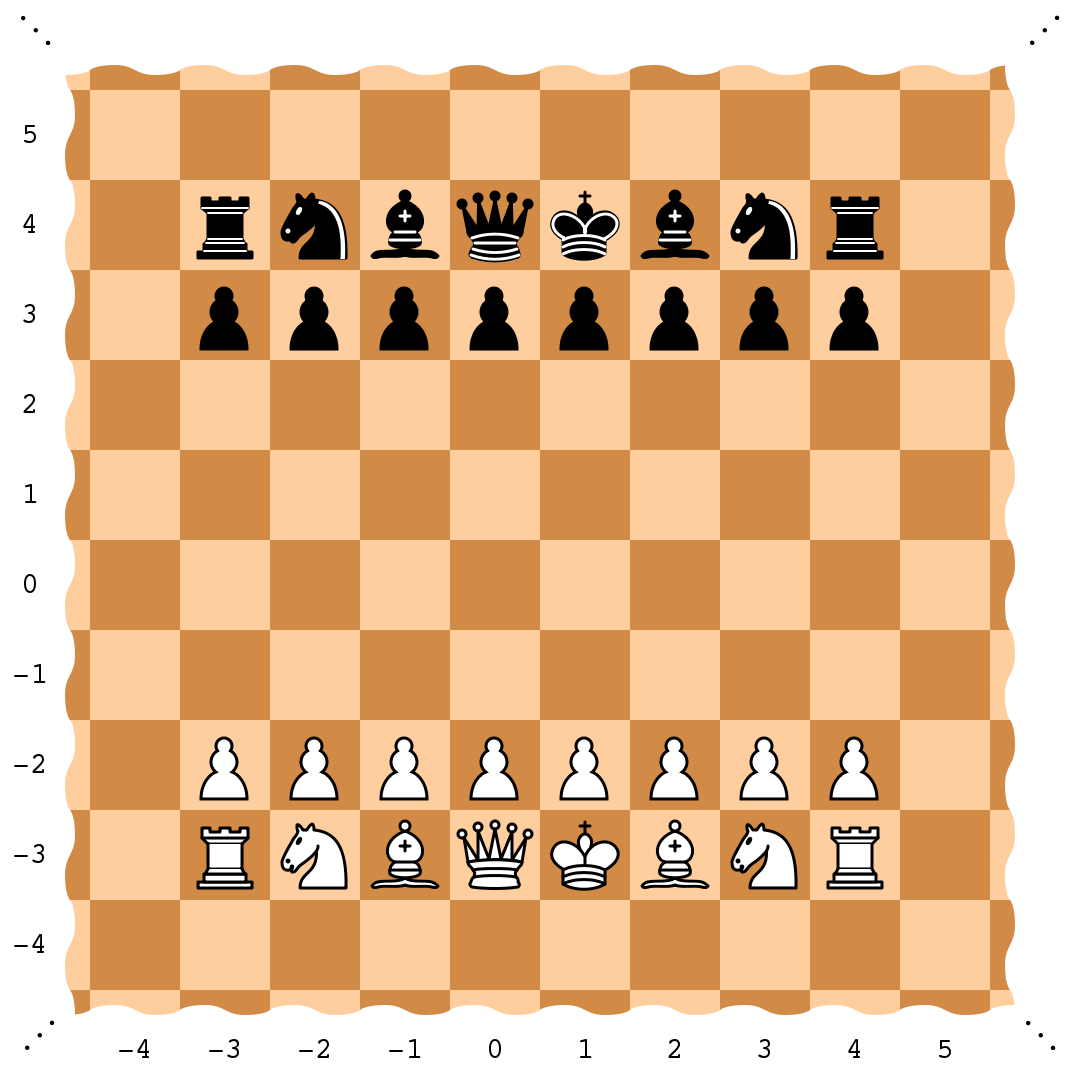
Let’s take a closer look at the countable non-standard models. It turns out that we can say a lot about their order type. Namely, all countable non standard models of PA have order type ω + (ω*+ω)·η. What does this notation mean? Let me break down each of the order types involved in that formula:
ω: order type of the naturals
ω*: order type of the negative integers
η: order type of the rationals
So ω*+ω is the order type of the integer line, and (ω*+ω)·η is the order type of a structure that resembles an integer line for each rational number. Thus, every countable non-standard model of PA looks like a copy of natural numbers followed by as many copies of integers as there are rational numbers. The order on this structure is lexicographic: two nonstandards on the same integer line are judged according to their position on the integer line, and two nonstandards on different integer lines are judged according to the position of these integer lines on the rational line. It’s not the easiest thing to visualize, but here’s my attempt:
Visualization of the order type of countable nonstandard models of Peano arithmetic
So if all countable non-standard models have the same order type, then where do they differ? It turns out that they differ in the details of how addition and multiplication work on the non-standards. (After all, a model of PA is defined by the size of its universe and its interpretation of ≤, +, and ×. Same order type means same ≤, so what’s left to vary is + and ×.) In each of the models, + and × work exactly like normal on the naturals. And + and × must operate on the non-standards in such a way as to maintain the truth of all the axioms of PA. So, for instance, since PA can prove that 2x = x + x, the same must be true for nonstandard x. And so on. But even given these restrictions, there are still uncountably many ways to define + and × on the non-standards.
What’s more, we have a theorem known as the Tennenbaum Theorem, which tells us that it’s impossible to give recursive definitions to + and × in non-standard models. Said more simply, addition and multiplication are uncomputable in every non-standard model of arithmetic!
One thing I remain unsure of is how the nonstandard models of Peano arithmetic compare to the structure of ω in nonstandard models of ZFC. We know that there must be models of ZFC where ω is nonstandard, by the compactness theorem (define ZFC* to be ZFC with an extra constant c, with the extra axioms “c ∈ ω”, “c ≠ 0”, “c ≠ 1”, “c ≠ 2”, and so on. ZFC* has a model by compactness, and this model is also a model of ZFC by monotonicity.) But is ZFC “better” at ruling out nonstandard models of the naturals than PA is? Or is there a nonstandard ω for every nonstandard model of Peano arithmetic?
I want to share a way to construct the order type of the Church-Kleene ordinal ω1CK. As far as I’m aware, this construction is original to me, and I think it’s much simpler and more elegant than others that I’ve found on the internet. Please let me know if you see any issues with it!
So, we start with the notion of a computable ordinal. A computable ordinal is a computable well-order on the natural numbers. In other words, it’s a well-order < on ℕ such that there exists a Turing machine that, given any two natural numbers n and m, outputs whether n < m according to that order.
There’s an injection from computable well-orders on ℕ to Turing machines, so there are countably many computable well-orders (at most one for each Turing machine). This means that there’s a list of all such computable well-orders. Let’s label the items on this list in order: {<0, <1, <2, <3, …}. Each <n stands for a Turing machine which takes in two natural number inputs and returns true or false based on the nth computable well-ordering.
Now, we want to construct a set with order type ω1CK. We’re going to have it be an order on the natural numbers, so what we have to work with from the start is the set {0, 1, 2, 3, 4, 5, 6, …}.
We start by splitting up this set into an infinite collection of sets. First, we take every other number, starting with 0: {0, 2, 4, 6, 8, …}. That’ll be our first set. We’ve left behind {1, 3, 5, 7, 9, …}, so next we take every other number from this set starting with 1: {1, 5, 9, 13, …}. Now we’ve left behind {3, 7, 11, 15, …}. Our next set, predictably, will be every other number from this set starting with 3. This is {3, 11, 19, 27, …}. And we keep on like this forever, until we’ve exhausted every natural number.
Now, we define our order to make everything in the first set less than everything in the second set, and everything in the second set less than everything in the third set, and so on. So far so good, but this only gives us order type ω2. Next we define the order WITHIN each set.
To do this, we’ll use our enumeration of computable orders. In particular, within the nth set, the ith number will be less than the jth number exactly in the case that i <n j. You can think about this as just treating each set “as if” it’s really {0, 1, 2, 3, …}, then ordering it according to <n, and then relabeling the numbers back to what they started as.
This fully defines our order. Now, what’s the order type of this set? Well, it can’t be any particular computable order type, because every computable order type can be found as a sub-order of it! So it must be some uncomputable order type. And by construction, we know it must be exactly the order type that contains all and only computable order types as suborders. But this is just the order type of the Church-Kleene ordinal!
So there we have it! We’ve constructed ω1CK. Now, remember that the Church-Kleene ordinal is uncomputable. But I just described an apparently well-defined process for creating an ordered set with its order! This means that some part of the process I described must be uncomputable. Challenge question for you: Which part is uncomputable, and can you think of a proof of its uncomputability that is independent of the uncomputability of ω1CK?
Last time we talked a little bit about some properties of the order type of ℚ. I want to go into more detail about these properties, and actually prove them to you. The proofs are nice and succinct, and ultimately rest heavily on the density of ℚ.
Every Countable Ordinal Can Be Embedded Into ℚ
Take any countable well-ordered set (X, ≺). Its order type corresponds to some countable ordinal. Since X is countable, we can enumerate all of its elements (the order in which we enumerate the elements might not line up with the well-order ≺). Let’s give this enumeration a name: (x1, x2, x3, …).
Now we’ll inductively define an order-preserving bijection from X into ℚ. We’ll call this function f. First, let f(x1) be any rational number. Now, assume that we’ve already defined f(x1) through f(xn-1) in such a way as to preserve the original order ≺. All we need to do to complete the proof is to assign to f(xn) a rational number such that the ≺ is still preserved.
Here’s how to do that. Split up the elements of X that we’ve already constructed maps for as follows: A = {xi | xi ≺ xn} and B = {xi | xi > xn}. In other words, A is the subset of {x1, x2, …, xn-1} consisting of elements less than x_n and B is the subset consisting of elements greater than xn. Every element of B is strictly larger than every element of A. So we can use the density of the rationals to find some rational number q in between A and B! We define f(xn) to be this rational q. This way of defining f(xn) preserves the usual order, because by construction, f(xn) < f(xi) for any i less than n exactly in the case that xn < xi.
By induction, then, we’ve guaranteed that f maps X to ℚ in such a way as to preserve the original order! And all we assumed about X was that it was countable and well-ordered. This means that any countable and well-ordered set can be found within ℚ!
No Uncountable Ordinals Can Be Embedded Into ℝ
In a well-ordered set X, every non-maximal element of X has an immediate successor (i.e. a least element that’s greater than it.) Proof: Take any non-maximal x ∈ X. Consider the subset of X consisting of all elements greater than x: {y ∈ X | x < y}. This set is not empty because α is not maximal. Any non-empty subset of a well-ordered set has a least element, so this subset has a least element. I.e, there’s a least element greater than x. Call this element S(x), for “the successor of x”,
Now, take any well-ordered subset X ⊆ ℝ (with the usual order). Since it’s well-ordered, every element has an immediate successor (by the previous paragraph). We will construct a bijection that maps X to ℚ, using the fact that ℚ is dense in ℝ (i.e. that there’s a rational between any two reals). Call this function f. To each element x ∈ X, f(x) will be any rational such that x < f(x) < S(x). This maps every non-maximal element of X to a rational number. To complete this, just map the maximal element of X to any rational of your choice. There we go, we’ve constructed a bijection from X to ℚ!
The implication of this is that every well-ordered subset of the reals is only countably large. In other words, even though ℝ is uncountably large, we can’t embed uncountable ordinals inside it! The set of ordinals we can embed within ℝ is exactly the set of ordinals we can embed within ℚ! (This set of ordinals is exactly ω1: the set of all countable ordinals).
Final Note
Notice that the previous proof relied on the fact that between any two reals you can find a rational. So this same proof would NOT go through for the hyper-reals! There’s no rational number (or real number, at that!) in between 1 and 1+ϵ. And in fact, you CAN embed ω1 into the hyperreals! This is especially interesting because the hyperreals have the same cardinality as the reals! So the embeddability of ω1 here is really a consequence of the order type of the hyperreals being much larger than the reals. And if we want to take a step towards even crazier extensions of ℝ, EVERY SINGLE ordinal can be embedded within the surreal numbers!
Take any set and place an order on it. If the order is a well-order (i.e. if every subset has a least element), then the set has the same order type as some particular ordinal. But the notion of order type can be extended beyond well-ordered sets. Any two ordered sets are said to have the same order type if they are order isomorphic: if there’s a bijective map f from one set to the other such that both f and f-1 preserve the ordering of elements.
One structure that has a very interesting order type is the rational numbers. After all, the rationals are a countable set, but every rational number resembles a “limit ordinal” in the sense that it has no immediate predecessor.
One question that we can ask to get some insight about the order type of the rational numbers is: what ordinals can be found within the rationals? That is, take some well-ordered subset of the rationals. Look at the order type of this subset. This order type corresponds to some ordinal. And different choices of well-ordered subsets of the rationals give us different ordinals! So which ordinals can we “find” within the rationals in this sense?
First off, every finite ordinal can obviously be found. To find the ordinal n, just take the subset {0, 1, 2, …, n-1}. We can also find ω! You can just take the subset {0, 1, 2, 3, …}. What about ω+1? Try for yourself: can you construct a subset of the rationals with the order type of ω+1?
There’s no unique way to do it, but one easy way is to take the subset {1/2, 3/4, 7/8, …, 1}. This set has a countable infinity of elements, one for each natural number, after all of which comes a single element: exactly the order type of ω+1!
If we want a subset of the rationals with order type ω+2, we can use the same trick: {1/2, 3/4, 7/8, …, 1, 2}. And clearly this extends for any ω+n. But how about ω+ω? Can you construct a subset of the rationals with this order type? (Do it yourself before reading on!)
Here’s one way: {1/2, 3/4, 7/8, …, 1+1/2, 1+3/4, 1+7/8, …}. It should be easy to see how to extend this trick to get ω⋅3, ω⋅4, and indeed ω⋅n for any finite n. You can even naturally extend this to get to ω⋅ω. But then what? Are we finished?
If you guessed no, you’re right! We can find subsets of the rationals with order type ω3, and ωn for any finite n, and ωω. (Try it!) And we can keep going beyond that as well. So how high can you go?
Turns out that EVERY countable ordinal can be embedded into the rationals, under the usual order! So in some sense the order type of the rationals is as complicated as possible while still being countable. Also, remember that the set of countable ordinals is uncountably large. So this means that the rationals are a countable ordered set that has all of the uncountably many countable ordinals embedded within it! Isn’t that great?
(One thing that makes this seem less insane is that when we’re looking at what ordinals can be embedded in the rationals, we’re searching through different subsets of the rationals. And even though the rationals are countable, the set of all subsets of the rationals is uncountably large.)
One more interesting thing: the set of all subsets of the rationals has cardinality ℶ1. But the set of all ordinals that can be embedded into the rationals is ω1, which has cardinality ℵ1. So if we start with the set of all subsets of the rationals, then strip away all but those that are well-ordered, and then choose just a single representative for each order type, we get a set of cardinality ℵ1. And there is no guarantee that this final set has the same cardinality as the original set, because this is the continuum hypothesis! This is a way to think about how to “construct” a real life set with cardinality ℵ1: look at the set of well-ordered subsets of the rationals, and split it into order-type equivalence classes.
What is an ordinal number? If you read my previous post, you might be convinced that an ordinal number is a particular type of set that contains all the ordinal numbers less than it. In particular, the ordinal 0 is the empty set, the ordinal 1 is the set {0}, the ordinal 2 is the set {0,1}, and so on. This is a fine way to think about ordinals, but there’s a much deeper view of them that I want to present in this post.
The fundamental concept is that of order types. Order types are to order-preserving bijections as cardinalities are to bijections. If you’ve seen pictures like these before, then they’re good to have in mind when you think about what order types are:
Let’s get into more detail about order types.
Take any two sets. If there is a bijection between them, then we say that they have the same cardinality. So we can think of each cardinal number as a class of sets, all in bijective correspondence with one another.
Take any two well-ordered sets. (Recall, a set is well-ordered if each of its subsets has a least element.) If there is an order-preserving bijection between them, then we say that the two sets have the same order type. So we can think of each ordinal number as a class of sets, all of the same order type.
For instance, the cardinal number “2” is the class of all sets with two elements (as all such sets are in bijective correspondence with one another). And the ordinal number “2” is the class of all well-ordered two-element sets. In particular, Von Neumann’s ordinal 2 = {0, 1} = {∅, {∅}} has this order type.
The finite cardinalities and finite order types line up nicely: any two well-ordered sets with the same finite cardinality are guaranteed to have the same order type. It’s in the realm of the infinite where order types and cardinalities come apart.
The cardinal number ℵ0 is the class of all sets that can be put into bijective correspondence with the set of natural numbers ω. This includes the set of even numbers and the set of rational numbers. So how many order types are there of sets with cardinality ℵ0?
Consider the following two ordered sets: X = {0 < 1 < 2 < 3 < …} and Y = {1 < 2 < 3 < … < 0}. They both have cardinality ℵ0, but do they have the same order types? If so, then there must be a bijection f: X → Y such that f is order-preserving (for all a ∈ X and b ∈ X, if a < b then f(a) < f(b)). But what element of X is mapped to 0 in Y? In the set Y, 0 is larger than every element besides itself, but there is no element of X that has this property! So no, X and Y do not have the same order types.
X is the order type of ω (a countably infinite list of elements with no elements that have infinitely many predecessors), and Y is the order type of ω+1 (a countably infinite list of elements with a single element coming after all of them). This tells us that there are at least two different order types within the cardinality ℵ0.
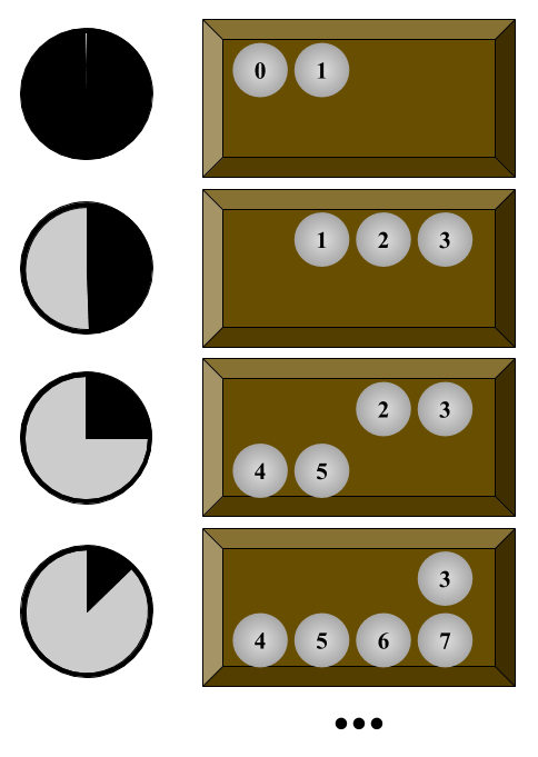
Can we construct an order on the set of natural numbers that has the same order type as ω+2? Well, all we need is for there to be two elements that are larger than all the rest. So we can write something like {2 < 3 < 4 < … < 0 < 1}. This generalizes easily to ω+n, for any finite n: {n+1 < n+2 < … < 0 < 1 < … < n} has the same order type as ω+n.
But now what about ω+ω, i.e. ω⋅2? To get a set of naturals with the same order type, we have to use a new trick. We need two countably infinite sequences of numbers that we can place beside one another. An easy way to accomplish this is by using the evens and odds: {0 < 2 < 4 < … < 1 < 3 < 5 < …}.
We can get an order on the naturals with the same order type as ω⋅2 + 1 by just choosing a single natural number to place after all the others. For instance: {2 < 4 < 6 < … < 1 < 3 < 5 < … < 0}. It should be easy to see how to get ω⋅2 + n for any finite n: just do {n < n+2 < n+4 < … < n+1 < n+3 < n+5 < … < 0 < 1 < 2 < … < n-1} And now how about ω⋅3?
(Try it out for yourself before reading on!)
To get ω⋅3, we need to place three countably infinite sequences of naturals side by side. For instance: {0 < 3 < 6 < … < 1 < 4 < 7 < … < 2 < 5 < 8 < …}.
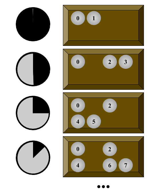
For ω⋅4, we can use a similar trick: {0 < 4 < 8 < … < 1 < 5 < 9 < … < 2 < 6 < 10 < … < 3 < 7 < 11 < …}. Again, we can quite easily generalize this to ω⋅n for any finite n: {0 < n < 2n < … < 1 < n+1 < 2n+1 < … < 2 < n+2 < 2n+2 < … < … < n-1 < 2n-1 < 3n-1 < …}. But how about ω⋅ω? How do we deal with ω2?
This is a fun exercise to try for yourself at home. Construct an order on the set of natural numbers that has the same order type as ω2. Then try to generalize the trick to get ω3, ω4, and ωn for any finite n.
Next construct an order on the naturals with the same order type as ωω! Can you do it for ω^ω^ω? And ω^ω^ω^…? One thing that should become clear is that the larger an ordinal you’re dealing with, the harder it becomes to construct an order on the naturals with the same order type. The natural question is: is it always possible to do this type of construction, or do we at some point run out of clever tricks to use to get to higher and higher countable ordinals?
Well, if an ordinal α is countable, then it is a well-ordered set with the same cardinality as the naturals. So there always exists some order that can be placed on the naturals to mimic the order type of α. But is this order always computable?
We call an order on the naturals computable if there’s some Turing machine which takes as input two naturals x and y and outputs whether x < y according to this order. We call an order type computable if there’s some computable order on the naturals with that order type. The standard order (0 < 1 < 2 < 3 < …) is computable, and it’s easy to see how to compute all the other orders we’ve discussed so far. But are ALL the countable order types computable?
The wonderful and strange answer is no. There are countable order types that are uncomputable! There must exist orders on the naturals with such order types, but these orders are so immensely complicated and strange that they cannot be defined by ANY Turing machine! Here’s a quick and easy proof of this. (The next three paragraphs are the coolest and most important part of this whole post, so pay attention!)
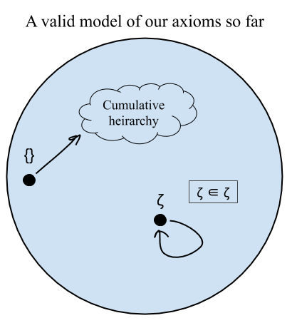
Turn your mind back to Von Neumann’s construction of the ordinals, according to which each ordinal was exactly the set of all smaller ordinals. More technically, a set α is a Von Neumann ordinal iff α is well ordered with respect to ∈ AND every element of α is also a subset of α. Consider now the set of all countable ordinals. It can be seen that this set is itself an ordinal. Can it be a countable ordinal? No, because if it were then it would have to be an element of itself! (This is not allowed in ZFC by the axiom of regularity.) This means that there are uncountably many countable ordinals.
Ok, so far so good. Now we just observe that there are only countably many Turing machines. So there are only countably many Turing machines that compute orders on the naturals. And therefore there are only countably many computable ordinals.
Putting this together, we see that there are uncountably many uncomputable countable order types (say that sentence out loud). After all, there are uncountably many countable ordinals, and only countably many computable ordinals!
And if there’s only countably many computable ordinals, then there’s some countable Von Neumann ordinal consisting of the set of all computable ordinals! This set couldn’t possibly be computable, because then it would be contained within itself. So it’s the smallest uncomputable ordinal! This set is called the Church-Kleene ordinal. Its order type is literally so convoluted and complex that no Turing machine can compute it!
Today I want to talk about ordinal numbers in ZFC set theory. VSauce does a great job introducing his viewers to the concepts of ordinal vs cardinal numbers, and giving a glimpse into the weird and wild world of mathematical infinity. I want to go a bit deeper, and show exactly how the ordinals are constructed in ZFC. Let’s begin!
Okay, so first of all, we’re talking about first-order ZFC, which is an axiomatic formalization of set theory in first-order logic. As a quick reminder, first order logic gives us access to the following alphabet of symbols: ( ) , ∧ ∨ ¬ → ↔ ∀ ∃ =, as well as an infinite store of variables (x, y, z, w, v, u, and so on). A first order language also includes a store of constant symbols, relation symbols, and function symbols.
For first-order set theory, we are going to add only a single extra-logical symbol to our alphabet: the “is-an-element-of” relation ∈. This is pretty remarkable when you consider that almost all of mathematics can be done with just ZFC! In some sense, you can give a pretty good description of mathematics as the study of the elementhood relation! Using just ∈ we can define everything we need, from ⊆ and ⋃ and ⋂ to the empty set ∅ and the power set function P(x). In fact, as we’ll see, we’re even going to define numbers using ∈!
The elementhood relation ∈ is given its intended meaning by the axiom of extensionality: ∀x∀y (x=y ↔ ∀z (z∈x ↔ z∈y)). In plain English this says that two sets are the same exactly when they have all the same elements.
The semantics of first order logic has two parts: a “universe” of individuals that are quantified over by ∀ and ∃, and an interpretation of each of the constant symbols (as individual objects in the universe), the relation symbols (as maps from the universe to truth values), and the function symbols (as maps from the universe to itself).
Our universe is going to be entirely composed of sets. This means that sets won’t be composed of non-set elements; the elements of non-empty sets are always themselves sets. And those sets themselves, if non-empty, are made out of sets. It’s sets all the way down!
Now, the topic of this essay is ordinal numbers in ZFC. So if everything in ZFC is a set, guess what ordinal numbers will be? You got it, sets! What sets? We can translate from ordinals to sets in a few words: the ordinal 0 is translated as the empty set, and every other ordinal is translated as the set of all smaller ordinals.
This tells us that 1 = {0}, 2 = {0, 1}, 3 = {0, 1, 2}, and so on. If we were to write these ordinals entirely in set notation, it would look like: ∅, {∅}, {∅,{∅}}, {∅,{∅},{∅,{∅}}}, and so on. The choice to associate these particular sets with the natural numbers is a convention introduced by John Von Neumann (it is, however, an exceedingly wise convention, and has many virtues that competing conventions do not have, as will become clearer once we ascend to the transfinite).
So, now we know that we are going to associate the finite ordinals with the empty set and supersets of the empty set. But of course, we haven’t yet even shown that the empty set exists in ZFC! To actually construct the empty set in ZFC, we have to add some more axioms. Let’s start with the obvious one: a sentence that asserts the existence of the empty set:
Axiom of Empty Set: ∃x∀y ¬(y∈x)
In other words, there’s some set x that contains no sets. Notice that we didn’t refer to the empty set by name. We can’t refer to it by name in our axioms, because we haven’t included any constant symbols in our language! To actually talk about the particular set ∅ (equivalently, 0), we can use the rule of existential instantiation, which allows us to remove any existential quantifier, as long as we change the name of the quantified variable to something that has not been previously used. So, for example, in any particular proof, we can do the following:
1. ∃x∀y ¬(y∈x) (Axiom of Empty Set)
2. ∀y ¬(y∈0) (from 1 by existential instantiation)
This is allowed so long as the symbol 0 has not appeared anywhere previously in the proof.
Now that we have the empty set, we need to be able to construct 1={0} and 2={0,1}. To do this, we introduce the axiom of pairing:
Axiom of Pairing: ∀x∀y∃z∀w (w∈z ↔ (w=x ∨ w=y))
This says that we can take any two sets x and y and form a new set z = {x, y}. We can right away use this axiom to construct the number 1.
We went from 3 to 4 by using universal instantiation (instantiating both variables x and y as 0), and from 4 to 5 by using existential instantiation (instantiating z as 1, which is allowed because we haven’t used the symbol 1 yet). The step from 5 to 6 is technically skipping a bunch of steps. Even though it’s obvious that we can replace (w=0 ∨ w=0) with w=0 inside the formula, there isn’t any particular rule of inference in first order logic that does it in one step. But since it is obvious that 5 semantically entails 6, and since first order logic has a sound and complete proof system, we know that 5 also syntactically entails 6.
To construct 2, we can simply use pairing again with 0 and 1:
We might think that we could simply use pairing once more to get 3 = {0,1,2}. But this won’t quite work. If we use pairing on 1 and 2 we get {1,2}, and if we use pairing again on this and 0 we get {0,{1,2}}, not {0,1,2}. In fact, we can easily see that any usage of pairing always produces a set with exactly two elements. And the set 3 has three elements! So pairing is not enough to get us where we want to go. To get to 3, we need a stronger axiom, which will allow us to take the union of sets.
Axiom of Union: ∀x∃y∀z (z∈y ↔ ∃w(z∈w ∧ w∈x))
This says that for any set x, we can construct a new set y which consists of the union of all sets in x. In other words, if z is an element of y, then z must be contained in some set w that’s an element of x.
Now, here’s how we’re going to construct 3. First we construct the set {2} by pairing 2 with itself. Then we construct the set {2,{2}} with pairing again. Then we union all the elements of this set to get 2⋃{2}. Now remember that 2 = {0,1}, so 2⋃{2} = {0,1}⋃{2} = {0,1,2}. And that’s 3!
Technically, we’ve now constructed 3. But let’s neaten this up and show that this set is really what we wanted (using more of the intuitive semantic arguments from before to skip many tedious steps).
We can construct 4 in pretty much the exact same way: first use pairing to construct {3} and then {3,{3}}, and then use union to construct 3⋃{3} = {0,1,2}⋃{3} = {0,1,2,3} = 4. I’ll go through this all formally one more time, more quickly than before:
It should be clear that this process can continue indefinitely. From the ordinal 4 we can construct 5 by taking the union of 4 and {4}, and from 5 we can construct 6 = 5⋃{5}. And so on. In fact, we can define the successor of any set x as exactly the set x⋃{x}: S(x) = x⋃{x}. And using the above construction, we know that this successor set will always exist!
Wonderful! So now we have an outline for the construction of every natural number. What’s next? What comes after 0, 1, 2, 3, 4, and so on? The first infinite ordinal, ω! Just as 4 is the set {0,1,2,3}, and 10 is the set of all the ordinals before it, ω is defined as exactly the set of all previous ordinals. In other words, ω is the set of all natural numbers! ω = {0,1,2,3,…}.
Now, how can we construct ω in ZFC? Can we do it using the axioms we have so far? You might be tempted to say something like “Sure! You’ve just demonstrated a process that constructs n+1 from any n, and we know how to construct 0 already. So don’t we already have the ability to construct all the natural numbers?”
Well, hypothetical you, it’s true that we now know how to construct each natural number. But constructing the infinite set containing all natural numbers is an entirely different matter. Remember that proofs are only allowed to be finitely long! So in any proof using only the methods we’ve used so far, we can only construct finitely many natural numbers (proportional to the length of the proof). To get ω, we need something more than the axioms we have so far. Introducing: the axiom of infinity!
But before we get there, I want to construct a handy bit of shorthand which will make what comes next a lot easier to swallow. What we’ll do is write out as a first-order sentence the assertion “x is the successor of y”, as well as the sentence “x is the empty set”, and then introduce a shorthand notation for them. Trust me, it will make life a lot easier.
First, “x is the successor of y”, which we can also write as “x = y⋃{y}”. Try this for yourself before reading on! Ok, now that you’re back, here it is: ∀z (z∈x ↔ (z∈y ∨ z=y)). We’ll call this sentence Succ(x,y). So if you ever see “Succ(x,y)” in the future, read it as “x is the successor of y” and know that if we wanted to be fully formal about it we could replace it with “∀z (z∈x ↔ (z∈y ∨ z=y))”.
Good! Now, let’s do the same with the sentence “x is the empty set”, which is the same thing as “x is 0”. Try it for yourself! And now, here it is: ∀y ¬(y∈x). We’ll call this sentence isZero(x).
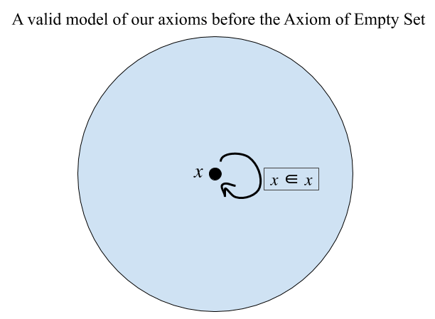
If this axiom looks like a lot to comprehend, imagine it without our shorthand! Conceptually, what’s going on with this axiom is actually pretty simple. We’re just asserting that there exists an infinite set x that contains 0, and that is closed under the successor operation. So this set is guaranteed to contain 0, as well as the successor of 0 (1), and the successor of the successor of 0 (2), and the successor of this (3), and so on forever. (Bonus question: what does the set theoretic universe look like if we remove the axiom of infinity and add its negation as an axiom instead? What mathematical structure is it isomorphic to?)
Quiz question for you: have we now constructed ω? That is, the axiom of of infinity does guarantee us the existence of a set, but are we sure that that set is exactly the set of natural numbers and nothing more?
The answer is no. The axiom of infinity does guarantee us the existence of an infinite set, and we know for sure that this set contains all the natural numbers, but there’s nothing guaranteeing that it doesn’t also contain other sets! To actually obtain ω, we need one more axiom. This axiom will be the most powerful one we’ve seen yet: the axiom of comprehension.
Axiom of Comprehension: ∀x∃y∀z (z∈y ↔ (z∈x ∧ φ(z)))
This tells us that for any set x, we can construct a new set y, which consists of exactly the elements of x that have a certain property φ. In set-builder notation, we can write: y = {z∈x: φ(z)}. (Bonus question: why do we have to define y as the subset of x that satisfies φ? Why not just say that there exists a set of all sets that satisfy φ? This unrestricted comprehension axiom appeared in the early formalizations of set theory, but there was a big problem with it. What was it?)
You may notice that there’s something different about this axiom than the previous ones. What’s up with that symbol φ(z)? Well, φ(z) is a stand-in for any well-formed formula in the language of ZFC, so long as φ contains only z as a free variable. What that means is that there’s actually not one single axiom of comprehension, but a countably infinite axiom schema, one for each well-formed formula φ.
For instance, we have as one instance of the axiom of comprehension that ∀x∃y∀z (z∈y ↔ (z∈x ∧ z=z)). As another instance of the axiom, we have ∀x∃y∀z (z∈y ↔ (z∈x ∧ z≠z)). Both of these are pretty trivial examples: in the first case the set y is exactly the same as x (as all sets are self-identical), and in the second case y is the empty set (as no set z satisfies the property z ≠ z). But we can do the same thing for any property whatsoever, so long as it can be encoded in a sentence of first-order ZFC. (Another bonus question: One of the axioms I’ve mentioned before has now been obviated by the introduction of these new axioms. Can you figure out which it is, and produce its derivation?)
We use the axiom of comprehension to “carve ω out” from the set whose existence is guaranteed by the axiom of infinity (remember, we already know for sure that this set contains all the natural numbers, it’s just that it might contain more elements as well). So what we need is to construct a sentence φ(z) such that the only set z that satisfies the sentence is the set of all natural numbers ω.
There are several such sentences. I’ll briefly present one simple one here. Again we’ll introduce a convenient shorthand for the sake of sanity. Take a look at this sentence that we saw earlier: “∀y ((isZero(y) → y∈x) ∧ (y∈x → ∃z (Succ(z,y) ∧ z∈x)))”. What this sentence says is that x is a superset of ω (it contains 0 and is closed under successorhood). So we’ll call this sentence “hasAllNaturals(x)”.
Now, we can write the following sentence: ∀x (hasAllNaturals(x) → z∈x).
Consider what this sentence says. It tells us that z is an element of every set that contains all the naturals. But one such set is the smallest set containing all the naturals, i.e. ω! So z must be an element of ω. In other words, z is a natural number. So this sentence will do for our definition of φ(z).
φ(z): ∀x (hasAllNaturals(x) → z∈x)
Just like with hasAllNaturals(z) and Succ(x,y) and isZero(x), you should read φ(z) as simply a shorthand for the above sentence. If we really wanted to torture ourselves with formality, we could write out the entire sentence using only the allowed symbols of first-order ZFC.
Now we can finally get ω. Let’s continue with our proof progression from earlier. We left off at 25, so:
In going from line 26 to 27, we gave the infinite set guaranteed us by the axiom of infinity a placeholder name, “inf”. Line 30 is what we’ve been aiming for for the last few hundred words, and it honestly looks a little underwhelming. It’s not so immediately clear from this line that ω has all the properties that we want of the natural numbers. But at the same time, we couldn’t write something like “∀z (z∈ω ↔ (z=0 ∨ z=1 ∨ z=2 ∨ …)), because first-order logic is finitary (we aren’t allowed infinitely long sentences). So we have to make do with a definition of ω that may look a little more abstract that we may like. Suffice it to say that line 30 really does serve as an adequate definition of ω. It tells us that ω is the smallest set that contains all natural numbers. From this, we can pretty easily show that any particular natural number is an element of ω, and (less easily) that any other set (say, the set {2} or {5,1}) is not an element of ω.
If you’ve followed so far, give yourself a serious pat on the back. Together we’ve ascended past the realm of the finite to our first transfinite ordinal. This is no small accomplishment. But our journey does not end here. In fact, it has only barely begun. We’re going to start picking up speed from here on out, because as you’ll see, the ground we have yet to cover is much much greater than the ground we’ve covered so far.
The first step is easy. We already saw earlier how you can construct for any set x its successor set x⋃{x}. This construction didn’t rely on our sets being finite, it works just as well for the set ω. So ω has a successor! We’ll call it ω+1! Don’t believe me? I’ll prove it to you:
And it doesn’t stop there: we can construct ω+2 = {0,1,2,3,…,ω,ω+1}. And ω+3 = {0,1,2,3,…,ω,ω+1,ω+2}. And so on, forever! By allowing the existence of one infinity, we’ve actually entailed the existence of an infinity of infinities!
But what’s next? We now have all the finite ordinals, and all the infinite ordinals of the form ω+n for finite n. What comes after this? Clearly, the next ordinal is just the set of all finite ordinals as well as all ordinals of the form ω+n! This ordinal is the smallest ordinal that’s larger than ω+n any finite n. So a natural name for it is ω+ω, or ω⋅2!
So conceptually ω⋅2 makes sense, but can we actually construct it? At first glance, this may seem unlikely. The axiom of infinity contains no guarantee that the infinite set it grants us contains ω, to say nothing of ω+1, ω+2, and the rest. And no finite amount of constructing successors will allow us to make the jump to ω⋅2 (for much the same reason as we needed the axiom of infinity to make the jump to ω). So perhaps we need to have a new axiom asserting the existence of ω⋅2? And then maybe we need a new axiom for ω⋅3, and ω⋅4, and so on forever! That would be a sad situation.
Well, things aren’t quite that bad. It turns out that we do need a new axiom. But we can do better than just guaranteeing the existence of ω⋅2. We’ll introduce an axiom schema that is by far the most powerful of all the axioms of ZFC. This axiom schema will take us far beyond ω⋅2, beyond ω⋅ω even, and far far beyond ω^ω and ω^ω^ω^… with infinitely many exponents. Introducing: the Axiom of Replacement! (dramatic music plays)
But first, we’re going to need to talk a little bit about the set theoretic notion of functions. I promise, it’ll be as quick as I can manage. Remember how we chose our language for ZFC to have no function symbols, only the single relation symbol ∈? This means that we have to build in functions through different means. We’ve already seen a hint of it when we talked about the sentence Succ(x,y) which said that x was the successor of y. This sentence is true for exactly the sets x and y such that x is the successor of y. We can think of the sentence as “selecting” ordered pairs (x,y) such that x = {y}. In other words, this sentence is filling the role of defining the function y ↦ {y}.
The same applies more generally. For any function f(x), we can construct the sentence F(x,y) which asserts “y = f(x)”. For instance, the identity function id(x) = x will be defined by the sentence Id(x,y): “y=x”. Notice that not all functions from sets to sets can be defined in this way, as we only have countably many sentences in our language to work with.
Suppose we’re handed a sentence φ(x,y). How are we to tell if φ(x,y) represents a function or just an ordinary sentence? Well, functions have the property that any input is mapped to exactly one output. We can write this formally: “∀x∀y∀z ((φ(x,y) ∧ φ(x,z)) → y=z)”. For shorthand, we’ll call this sentence isAFunction(φ).
And now we’re ready for the axiom schema of replacement.
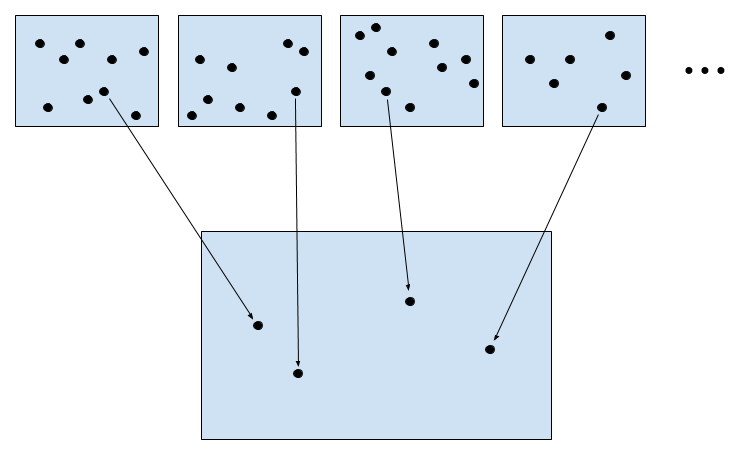
In English, this says that for any definable function f (defined by φ), and for any set of inputs x, the image of x under f exists. Like with the axiom schema of comprehension, this is a countably infinite collection of axioms, one for each well formed formula φ(w,z).
Let’s use this axiom to construct ω⋅2. First we define a function f that takes any finite number n to the ordinal ω+n. (Challenge: Try to explicitly define this function! Notice that the most obvious method for defining the function requires second-order logic. Try to come up with a trick that allows it to be defined in first-order ZFC!) Then we prove that this really is a function. Then we apply the axiom of replacement with our domain as ω (the set of all natural numbers). The image of ω under f is the set {ω,ω+1,ω+2,ω+3,…}. Not quite what we want. But we’re almost there!
Next we use the axiom of pairing to pair this newly constructed set with ω itself, giving us {{0,1,2,…}, {ω,ω+1,ω+2,…}}. And finally, we apply the axiom of union to this set, giving us {0,1,2,…,ω,ω+1,ω+2,…} = ω⋅2!
Phew, that was a lot of work just to make the jump to from ω to ω⋅2. But it was worth it! Now we can also jump to ω⋅3 in the exact same way!
Define a function f that maps n to ω⋅2+n. Now use replacement with ω as the domain to construct the set {ω⋅2, ω⋅2+1, ω⋅2+2, …}. Pair this set with ω⋅2, and union the result. This gives ω⋅3!
In exactly the same way, we can use the axiom of replacement to get ω⋅4, ω⋅5, ω⋅6, and so on to ω⋅n for any finite n! But it doesn’t stop there. We’ve just described a procedure to get ω⋅n for any finite n. So we write it as a function!
Define f as the function that maps n to ω⋅n. Now use replacement of f with ω as the domain to get the set {0, ω, ω⋅2, ω⋅3, ω⋅4, ω⋅5, …}. Apply the axiom of union to this set, and what do you get? Well it has to contain ω⋅n for every finite n, since each ω⋅n is contained in ω⋅m for every larger m. So it’s larger than all ordinals of the form ω⋅n for finite n. This new ordinal we’ve constructed is called ω⋅ω, or ω2.
But of course, our journey doesn’t stop there. We can use replacement to generate ω2 + ω, and ω2 + ω⋅2, ω2 + ω⋅3, and so on. But we can go further and use replacement to generate ω2 + ω2, or ω2⋅2! And from there we get ω2⋅3, ω2⋅4, and so on. And applying replacement to the function from n to ω2⋅n, we get a new ordinal larger than everything before, called ω3.
As you might be suspecting, this goes on forever. We can continually apply the axiom of replacement to get mind-bogglingly large infinities, each greater than the last. But here’s the kicker: all of these infinite ordinals that we’ve created so far? They all have the samecardinality.
Yes, that’s right. You may have thought that we had transcended ω in cardinality long ago, but no. For each infinite ordinal we’ve created so far, there’s a one-to-one mapping between it and ω. Think about it: every time we used replacement, we constructed a function that mapped an existing ordinal to a new one of the same cardinality. And in applying replacement to this function, we guaranteed that the new ordinal we created cannot be a larger cardinality than the existing ordinal! So each time we use replacement with a countable domain, we get a new countable set, each of whose elements is countable. And then if we use pairing or union, we’re always going to stay in the domain of the countable (unioning two countable sets just gets you another countable set, as does unioning a countable infinity of countable sets).
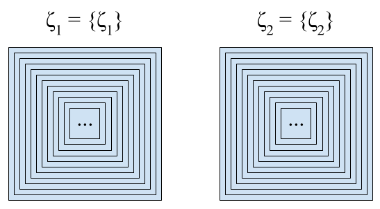
So now turn your mind to the following set: the set of all countable ordinals. Is this set itself an ordinal? It is if it’s the smallest uncountable ordinal, as then it contains every ordinal smaller than itself by definition! And what’s the cardinality of this set? It can’t be countable, because then it would have to be an element of itself! (Bonus question: Why is it that no ordinal can be an element of itself? Use the axiom of extensionality! Bonus question 2: In general, no set can be an element of itself. But this is not guaranteed by the axioms I’ve presented so far. The axiom that does the job is called the axiom of regularity/foundation, and it says that every set must have an element that it is disjoint with. Why does this prevent us from having sets that contain themselves?)
So this ordinal is the first uncountable ordinal. Its name is ω1. The cardinality of ω1 is the smallest cardinality that follows the cardinality of ω, and it’s called “aleph one” and written א1.
Now, I’ve already said that the same old paradigm we’ve used so far can’t get us to ω1. So can we get there with ZFC? It turns out that the answer is yes, and at the moment I’m not quite sure exactly how. It turns out that not only can ZFC construct ω1, it can also construct ω2 (the first ordinal with a larger cardinality than ω1), ω3, ω4, and so on forever.
So does ZFC have any limits? Or can we in principle construct every ordinal, using ever more ingenious means to transcend the limitations of our previous paradigms? The answer is no: ZFC is limited. There are ordinals so large that even ZFC cannot prove their existence (these ordinals have what’s called inaccessible cardinalities). To construct these new infinities, we must add them in as axioms, just as we had to for infinity (and indeed, for 0).
One might think that when we get to ordinals that are this mind-bogglingly large, nothing of any consequence could follow from asserting their existence. But this is not the case! Remarkably, if you add these new infinities to your theory, you can prove the consistency of ZFC. (That is, the consistency of the theory I’ve presented so far, which does not have these large cardinal axioms.) And to prove the consistency of this new theory, you must add even larger infinities. And now to prove the consistency of this one, you must expand the universe of sets again! And so on forever.
One might ask: “So how big is the universe of sets really?” At what point do we content ourselves to stop axiomatically asserting new and larger infinities, and say that we’ve obtained an adequate formalization of what the universe of sets looks like? I’m really not sure how to think about this question. Anyway, next up will be ordinal notation, and the notion of computable ordinals!
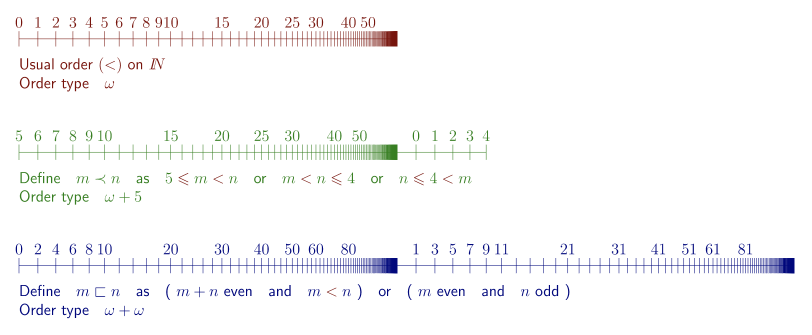
There are some chess positions in which one player can force a win. Here’s an extremely simple example:
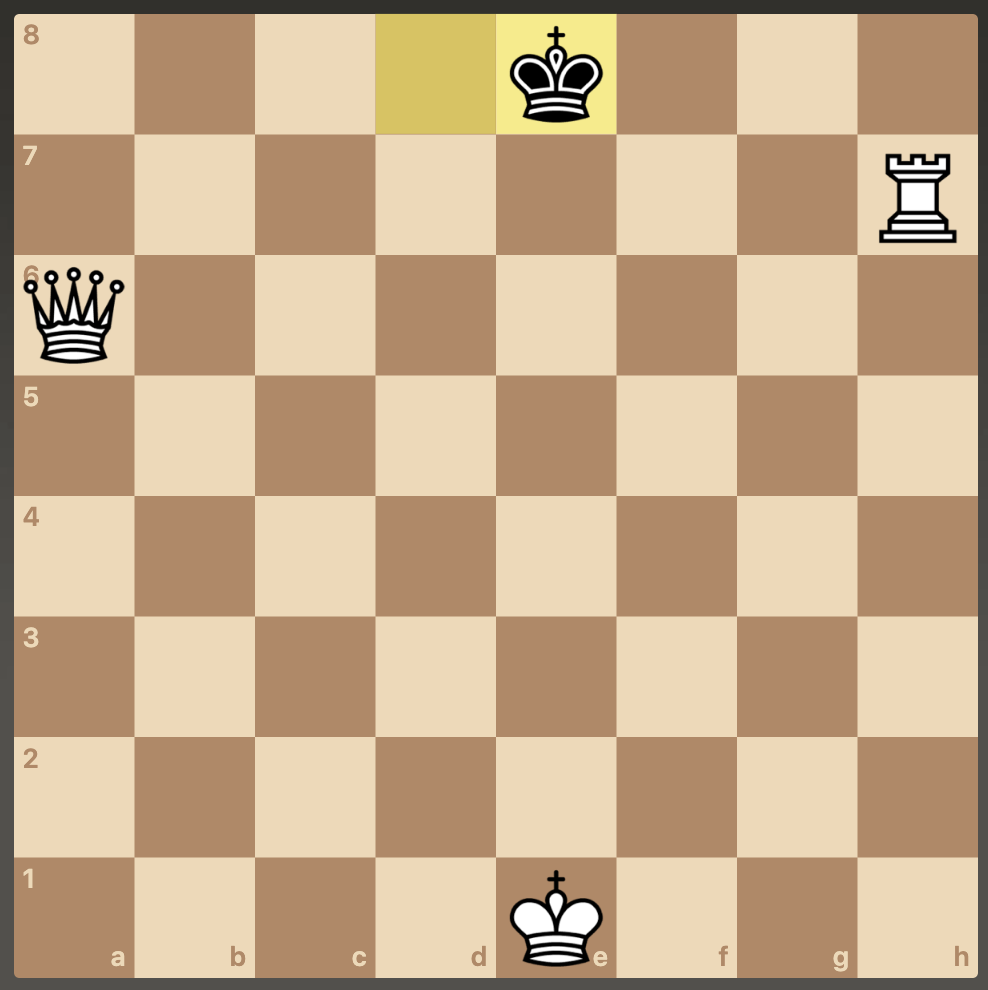
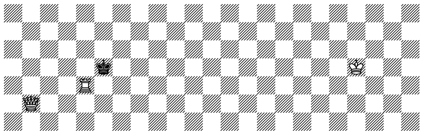
White just moves their queen up to a8 and checkmates Black. Some winning positions are harder to see than this. Take a look at the following position. Can you find a guaranteed two-move checkmate for White?
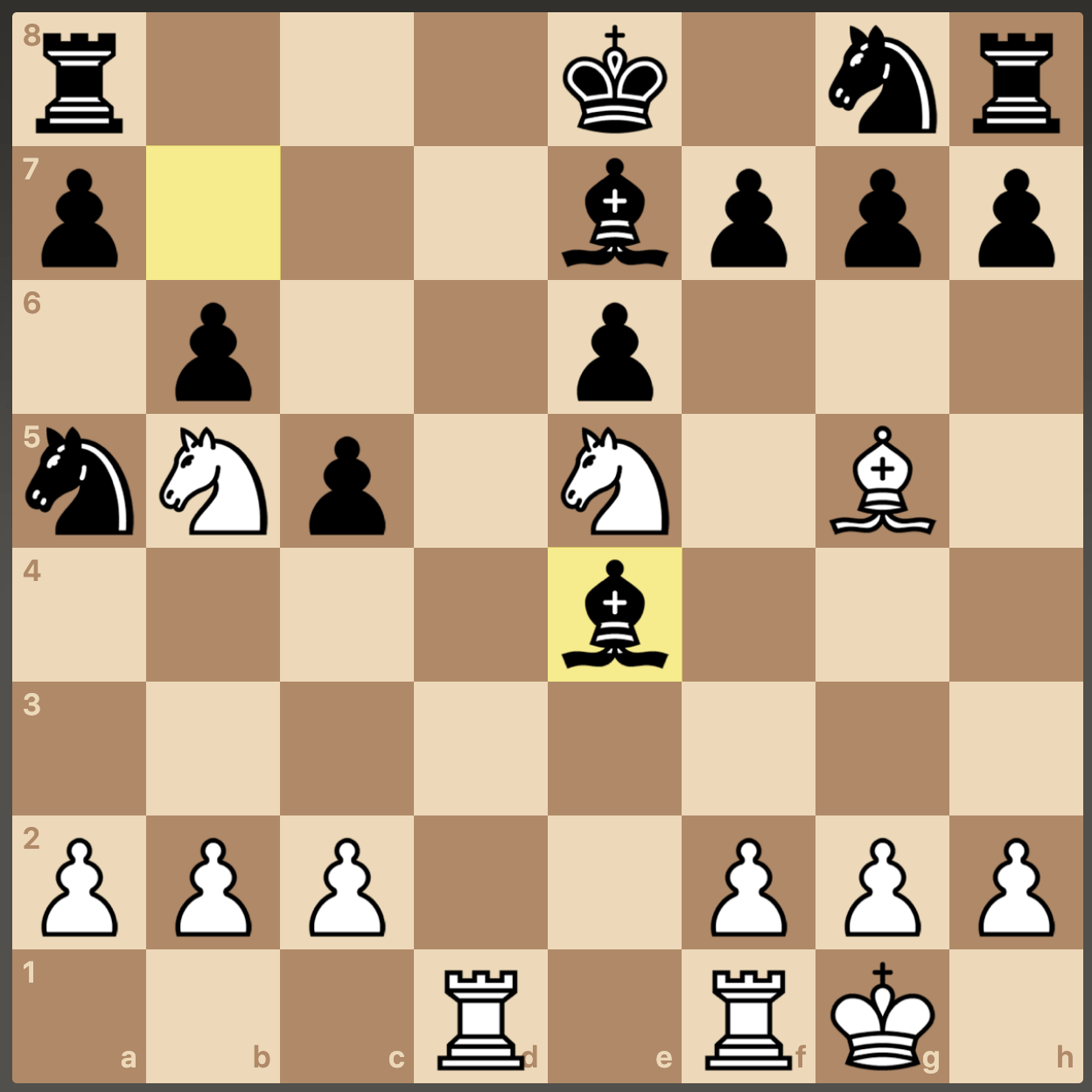
And for fun, here’s a harder one, again a guaranteed two-move checkmate, this time by Black:
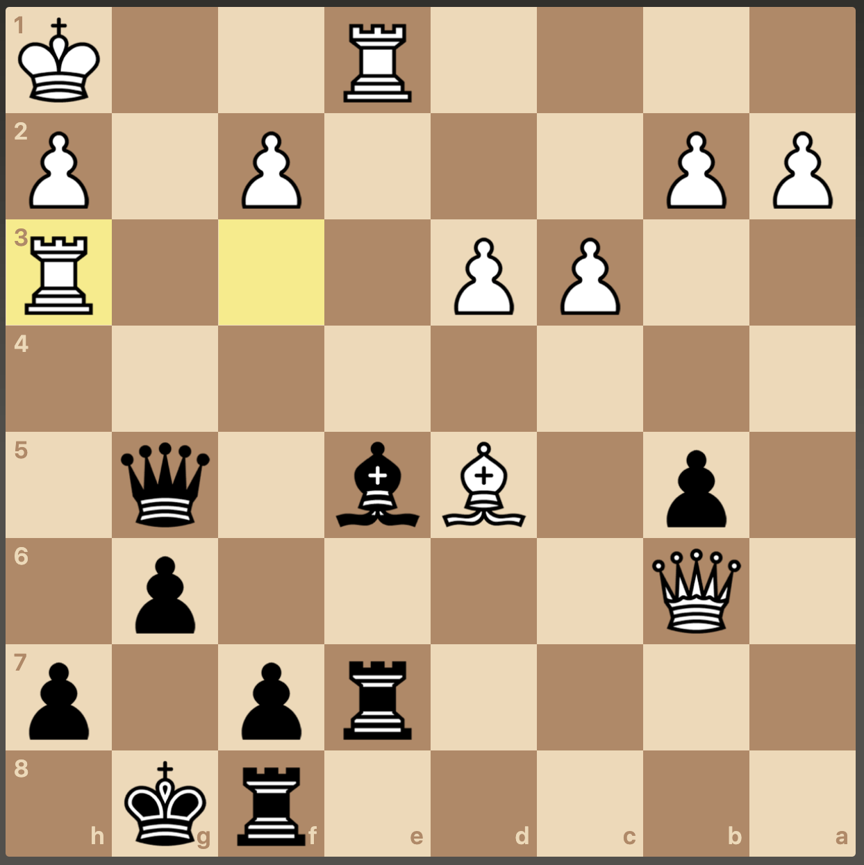
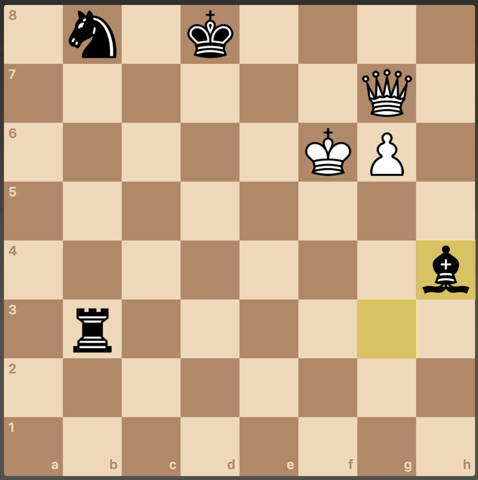
Notice that in this last one, the opponent had multiple possible moves to choose from. A forced mate does not necessarily mean restricting your opponent to exactly one move on each of their turns. It just means that no matter what they do, you can still guarantee a win. (Edit: with best play from White, this is not actually a forced mate.) Forced wins can become arbitrarily complicated and difficult to see if you’re looking many moves down the line, as you have to consider all the possible responses your opponent has at each turn. The world record for the longest forced win is the following position:
It’s White’s move, and White does have a strategy for a forced win. It just takes 549 turns to actually do this! (This strategy does violate the 50-move rule, which says that after 50 turns with no pawn moves or capture the game is drawn.) At this link you can watch the entire 549 move game. Most of it is totally incomprehensible to human players, and apparently top chess players that look at this game have reported that the reasoning behind the first 400 moves is opaque to them. Interestingly, White gets a pawn promotion after six moves, and it promotes it to a knight instead of a queen! It turns out that promoting to a queen actually loses for White, and their only way to victory is the knight promotion!
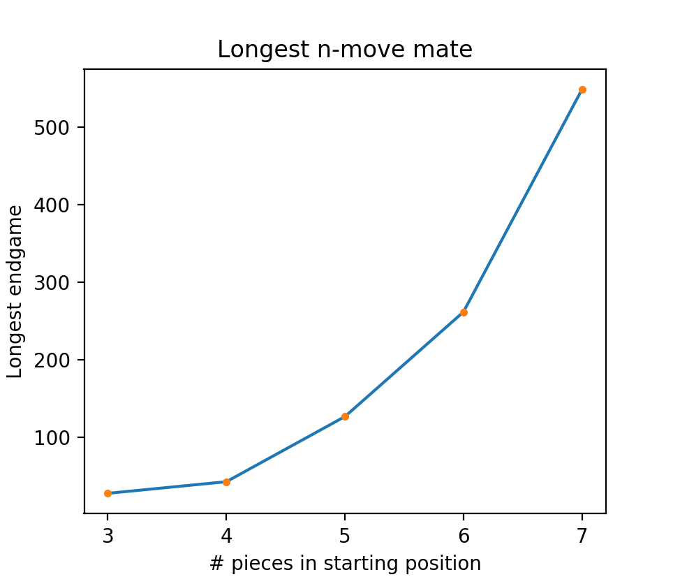
This position is the longest forced win with 7 pieces on the board. There are a few others that are similarly long. All of them represent a glimpse at the perfect play we might expect to see if a hypercomputer could calculate the whole game tree for chess and select the optimal move.
A grandmaster wouldn’t be better at these endgames than someone who had learned chess yesterday. It’s a sort of chess that has nothing to do with chess, a chess that we could never have imagined without computers. The Stiller moves are awesome, almost scary, because you know they are the truth, God’s Algorithm – it’s like being revealed the Meaning of Life, but you don’t understand one word.
Tim Krabbe
With six pieces on the board, the longest mate takes 262 moves (you can play out this position here). For five pieces, it’s 127 moves, for four it’s 43 moves, and the longest 3-man mate takes 28 moves.
But now a natural question arises. We know that a win can be forced in some positions. But how about the opening position? That is, is there a guaranteed win for White (or for Black) starting in this position?
Said more prosaically: Can chess be solved?
Zermelo’s theorem, published in “On an Application of Set Theory to the Theory of the Game of Chess” (1913), was the first formal theorem in game theory. It predated the work of von Neumann (the so-called “father of game theory”) by 15 years. It proves that yes, it is in fact possible to solve chess. We don’t know what the solution is, but we know that either White can force a win, or Black can force a win, or the result will be a draw if both play perfectly.
Of course, the guarantee that in principle there is a solution to chess doesn’t tell us much in practice. The exponential blowup in the number of possible games is so enormous that humans will never find this solution. Nonetheless, I still find it fascinating to think that the mystery of chess is ultimately a product of computational limitations, and that in principle, if we had a hypercomputer, we could just find the unique best chess game and watch it play out, either to a win by one side or to a draw. That would be a game that I would love to see.
✯✯✯
Here’s another fun thing. There’s an extremely bizarre variant on chess called suicide chess (or anti-chess). The goal of suicide chess is to lose all your pieces. Of course, if all the rules of play were the same, it would be practically impossible to win (since your opponent could always just keep refusing to take a piece that you are offering them). To remedy this, in suicide chess, capturing is mandatory! And if you have multiple possible captures, then you can choose among them.
Suicide chess gameplay is extremely complicated and unusual looking, and evaluating who is winning at any given moment tends to be really difficult, as sudden turnarounds are commonplace compared to ordinary chess. But one simplifying factor is that it tends to be easier to restrict your opponents’ moves. In ordinary chess, you can only restrict your opponents’ moves by blocking off their pieces or threatening their king. But in suicide chess, your opponents’ moves are restricted ANY time you put one of your pieces in their line of fire! This feature of the gameplay makes the exponential blow up in possible games more manageable.
Given this, it probably won’t be much of a surprise that suicide chess is, just like ordinary chess, in principle solvable. But here’s the crazy part. Suicide chess is solved!!
That’s right: it was proven a triple of years ago that White can force a win by moving first with e3!
Here’s the paper. The proof amounts to basically running a program that looks at all possible responses to e3 and expands out the game tree, ultimately showing that all branches can be terminated with White losing all pieces and winning the game.
Not only do we know that by starting with e3, White is guaranteed a win, we also know that Black can force a win if White starts with any of the following moves: a3, b4, c3, d3, d4, e4, f3, f4, h3, h4, Nc3, Nf3. As far as I was able to tell, there are only six opening moves remaining for which we don’t know if White wins, Black wins, or they draw: a4, b3, c4, e3, g3, and g4.
✯✯✯
Alright, final chess variant trivia. Infinite chess is just chess, but played on an infinite board.
There’s a mind-blowing connection between infinite chess and mathematical logic. As a refresher, a little while back I discussed the first-order theory of Peano arithmetic. This is the theory of natural numbers with addition and multiplication. If you recall, we found that Peano arithmetic was incomplete (in that not all first-order sentences about the natural numbers can be proven from its axioms). First order PA is also undecidable, in that there exists no algorithm that takes in a first order sentence and returns whether it is provable from the axioms. (In fact, first order logic in general is undecidable! To get decidability, you have to go to a weaker fragment of first order logic known as monadic predicate calculus, in which predicates take only one argument and there are no functions. As soon as you introduce a single binary predicate, you lose decidability.)
Okay, so first order PA (the theory of natural numbers with addition and multiplication) is incomplete and undecidable. But there are weaker fragments of first order PA that are decidable! Take away multiplication, and you have Presburger arithmetic, the theory of natural numbers with addition. Take away addition, and you have Skolem arithmetic, the theory of natural numbers with multiplication. Both of these fragments are significantly weaker than Peano arithmetic (each is unable to prove general statements about the missing operation, like that multiplication is commutative for Presburger arithmetic). But in exchange for this weakness, you get both decidability and completeness!
How does all this relate to infinite chess? Well, consider the problem of determining whether there exists a checkmate in n turns from a given starting position. This seems like a really hard problem, because unlike in ordinary chess, now it’s possible for there to be literally infinite possible moves for a given player from a position. (For instance, a queen on an empty diagonal can move to any of the infinite locations on this diagonal.) So apparently, the game tree for infinite chess, in general, branches infinitely. Given this, we might expect that this problem is not decidable.
Well, it turns out that any instance of this problem (any particular board setup, with the question of whether there’s a mate-in-n for one of the players) can be translated into a sentence in Presburger arithmetic. You do this by translating a position into a fixed length sequence of natural numbers, where each piece is given a sequence of numbers indicating its type and location. The possibility of attacks can be represented as equations about these numbers. And since the distance pieces (bishops, rooks, and queens – those that have in general an infinite number of available moves) all move in straight lines, there are simple equations expressible in Presburger arithmetic that describe whether these pieces can attack other pieces! From the attack relations, you can build up more complicated relations, including the mate-in-n relation.
So we have a translation from the mate-in-n problem to a sentence in Presburger arithmetic. But Presburger arithmetic is decidable! So there must also be a decision procedure for the mate-in-n problem in infinite chess. And not only is there a decision procedure for the mate-in-n problem, but there’s an algorithm that gives the precise strategy that achieves the win in the fewest number of moves!
Here’s the paper in which all of this is proven. It’s pretty wild. Many other infinite chess problems can be proven to be decidable by the same method (demonstrating interpretability of the problem in Presburger arithmetic). But interestingly, not all of them! This has a lot to do with the limitations of first-order logic. The question of whether, in general, there is a forced win from a given position can not be shown to be decidable in this way. (This relates to the general impossibility in first-order logic of expressing infinitely long statements. Determining whether a given position is a winning position for a given player requires looking at the mate-in-n problem, but without any upper bound on what this n is – on how many moves the win may take.) It’s not even clear whether the winning-position problem can be phrased in first-order arithmetic, or whether it requires going to second-order!
The paper takes this one step further. This proof of the decidability of the mate-in-n problem for infinite chess doesn’t crucially rest upon the two-dimensionality of the chess board. We could easily translate the proof to a three-dimensional board, just by changing the way we code positions! So in fact, we have a proof that the mate-in-n problem for k-dimensional infinite chess is decidable!
I’ll leave you with this infinite chess puzzle:
It’s White’s turn. Can they guarantee a checkmate in 12 moves or less?
Last post I described the Ross-Littlewood paradox, in which an ever-expanding quantity of numbered billiard balls are placed into a cardboard box in such a way that after an infinite number of steps the box ends up empty. Here’s a version of this paradox:
Process 1 Step 1: Put 1 through 9 into the box.
Step 2: Take out 1, then put 10 through 19 into the box.
Step 3: Take out 2, then put 20 through 29 into the box.
Step 4: Take out 3, then put 30 through 39 into the box.
And so on.
Box contents after each step Step 1: 1 through 9 Step 2: 2 through 19 Step 3: 3 through 29
Step 4: 4 through 39
And so on.
Now take a look at a similar process, where instead of removing balls from the box, we just change the number that labels them (so, for example, we paint a 0 after the 1 to turn “Ball 1” to “Ball 10″).
Process 2 Step 1: Put 1 through 9 into the box
Step 2: Change 1 to 10, then put 11 through 19 into the box.
Step 3: Change 2 to 20, then put 21 through 29 in.
Step 3: Change 3 to 30, then put 31 through 39 in.
And so on.
Box contents after each step Step 1: 1 through 9
Step 2: 2 through 19
Step 3: 3 through 29
Step 4: 4 through 39
And so on.
Notice that the box contents are identical after each step. If that’s all that you are looking at (and you are not looking at what the person is doing during the step), then the two processes are indistinguishable. And yet, Process 1 ends with an empty box, and Process 2 ends with infinitely many balls in the box!
Why does Process 2 end with an infinite number of balls in it, you ask?
Process 2 ends with infinitely many balls in the box, because no balls are ever taken out. 1 becomes 10, which later becomes 100 becomes 1000, and so on forever. At infinity you have all the natural numbers, but with each one appended an infinite number of zeros.
So apparently the method you use matters, even when two methods provably get you identical results! There’s some sort of epistemic independence principle being violated here. The outputs of an agent’s actions should be all that matters, not the specific way in which the agent obtains those outputs! Something like that.
Somebody might respond to this: “But the outputs of the actions aren’t the same! In Process 1, each step ten are added and one removed, whereas in Process 2, each step nine are added. This is the same with respect to the box, but not with respect to the rest of the universe! After all, those balls being removed in Process 1 have to go somewhere. So somewhere in the universe there’s going to be a big pile of discarded balls, which will not be there in Process 2.
This responds holds water as long as our fictional universe doesn’t violate conservation of information, as if not, these balls can just vanish into thin air, leaving no trace of their existence. But that rebuttal feels cheap. Instead, let’s consider another variant that gets at the same underlying problem of “relevance of things that should be irrelevant”, but avoids this problem.
Process 1 (same as before)
Step 1: Put 1 through 9 into the box.
Step 2: Take out 1, then put 10 through 19 into the box.
Step 3: Take out 2, then put 20 through 29 into the box.
Step 4: Take out 3, then put 30 through 39 into the box.
And so on.
Box contents after each step Step 1: 1 through 9
Step 2: 2 through 19
Step 3: 3 through 29
Step 4: 4 through 39
And so on.
And…
Process 3 Step 1: Put 1 through 9 into the box.
Step 2: Take out 9, then put 10 through 19 into the box.
Step 3: Take out 19, then put 20 through 29 into the box.
Step 4: Take out 29, then put 30 through 39 into the box.
And so on.
Box contents after each step Step 1: 1 through 9
Step 2: 1 to 8, 10 to 19
Step 3: 1 to 8, 10 to 18, 20 to 29
Step 4: 1 to 8, 10 to 18, 20 to 28, 30 to 39
And so on
Okay, so as I’ve written it, the contents of each box after each step are different in Processes 1 and 3. Just one last thing we need to do: erase the labels on the balls. The labels will now just be stored safely inside our minds as we look over the balls, which will be indistinguishable from one another except in their positions.
Now we have two processes that look identical at each step with respect to the box, AND with respect to the external world. And yet, the second process ends with an infinite number of balls in the box, and the first with none! (Every number that’s not one less than a multiple of ten will be in there.) It appears that you have to admit that the means used to obtain an end really do matter.
But it’s worse than this. You can arrange things so that you can’t tell any difference between the two processes, even when observing exactly what happens in each step. How? Well, if the labelling is all in your heads, then you can switch around the labels you’ve applied without doing any harm to the logic of the thought experiment. So let’s rewrite Process 3, but fill in both the order of the balls in the box and the mental labelling being used:
Process 3 Start with:
1 2 3 4 5 6 7 8 9
Mentally rotate labels to the right:
9 1 2 3 4 5 6 7 8
Remove the furthest left ball:
1 2 3 4 5 6 7 8
Add the next ten balls to the right in increasing order:
1 2 3 4 5 6 7 8 10 11 12 13 14 15 16 17 18 19
Repeat!
Compare this to Process 1, supposing that it’s done without any relabelling:
Process 1 Start with:
1 2 3 4 5 6 7 8 9
Remove the furthest left ball:
2 3 4 5 6 7 8 9
Add the next tell balls to the right in increasing order:
2 3 4 5 6 7 8 9 10 11 12 13 14 15 16 18 19
Repeat!
If the labels are all in your head, then these two processes are literally identical except for how a human being is thinking about them.
But looking at Process 3, you can prove that after Step 1 there will always be a ball labelled 1 in the box. Same with 2, 3, 4, and all other numbers that are not a multiple of 10 minus one. Even though we remove an infinity of balls, there are ball numbers that are never removed. And if we look at the pile of discarded balls, we’ll see that it consists of 9, 19, 29, 39, and so on, but none of the others. Unless some ball numbers vanish in the process (which they never do!), all the remainders must still be sitting in the box!
So we have two identical-in-every-relevant-way processes, one of which ends with an infinite number of balls in the box and the other with zero. Do you find this troubling? I find this very troubling. If we add some basic assumption that an objective reality exists independent of our thoughts about it, then we’ve obtained a straightforward contradiction.
✯✯✯
Notice that it’s not enough to say “Well, in our universe this process could never be completed.” This is for two reasons:
First of all, it’s actually not obvious that supertasks (tasks involving the completion of an infinite number of steps in a finite amount of time) cannot be performed in our universe. In fact, if space and time are continuous, then every time you wave your hand you are completing a sort of supertask.
You can even construct fairly physically plausible versions of some of the famous paradoxical supertasks. Take the light bulb that blinks on and off at intervals that get shorter and shorter, such that after some finite duration it has blinked an infinity of times. We can’t say that the bulb is on at the end (as that would seem to imply that the sequence 0101010… had a last number) or that it is off (for much the same reason). But these are the only two allowed states of the bulb! (Assume the bulb is robust against bursting and all the other clever ways you can distract from the point of the thought experiment.)
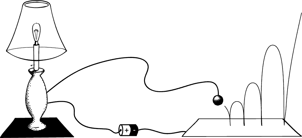
Now, here’s a variant that seems fairly physically reasonable:
A ball is dropped onto a conductive plate that is attached by wire to a light bulb. The ball is also wired to the bulb, so that when the ball contacts the plate, a circuit is completed that switches the light bulb on. Each bounce, the ball loses some energy to friction, cutting its velocity exactly in half. This means that after each bounce, the ball hangs in the air for half as long as it did the previous bounce.
Suppose the time between the first and second bounce was 1 second. Then the time between the second and third will be .5 seconds. And next will be .25 seconds. And so on. At 2 seconds, the ball will have bounced an infinite number of times. So at 2 seconds, the light bulb will have switched on and off an infinite number of times.
And of course, at 2 seconds the ball is at rest on the plate, completing the circuit. So at 2 seconds, upon the completion of the supertask, the light will be on.
Notice that there are no infinite velocities here, or infinite quantities of energy. Just ordinary classical mechanics applied to a bouncing ball and a light bulb. What about infinite accelerations? Well even that is not strictly speaking necessary; we just imagine that each velocity reversal takes some amount of time, which shrinks to zero as the velocity shrinks to zero in such a way as to keep all accelerations finite and sum to a finite total duration.
All this is just to say that we shouldn’t be too hasty in dismissing the real-world possibility of apparently paradoxical supertasks.
But secondly, and more importantly, physical possibility is not the appropriate barometer of whether we should take a thought experiment seriously. Don’t be the person that argues that the fat man wouldn’t be sufficient to stop a trolley’s momentum. When we find that some intuitive conceptual assumptions lead us into trouble, the takeaway is that we need to closely examine and potentially revise our concepts!
Think about Russell’s paradox, which showed that some of our most central intuitions about the concept of a set lead us to contradiction. Whether or not the sets that Bertie was discussing can be pointed to in the physical world is completely immaterial to the argument. Thinking otherwise would have slowed down progress in axiomatic set theory immensely!
These thought experiments are a problem if you believe that it is logically possible for there to be a physical universe in which these setups are instantiated. That’s apparently all that’s required to get a paradox, not that the universe we live in happens to be that one.
So it appears that we have to conclude some limited step in the direction of finitism, in which we rule out a priori the possibility of a universe that allows these types of supertasks. I’m quite uncomfortable with this conclusion, for what it’s worth, but I don’t currently see a better option.
You have in front of you an empty box. You also have on hand an infinite source of billiard balls, numbered 0, 1, 2, 3, 4, and so on forever.
At time zero, you place balls 0 and 1 in the box.
In thirty minutes, you remove ball 0 from the box, and place in two new balls (2 and 3).
Fifteen minutes after that, you remove ball 1 from the box, and place in two new balls (4 and 5).
7.5 minutes after that, you remove ball 2 and place in balls 6 and 7.
And so on.
After an hour, you will have taken an infinite number of steps. How many billiard balls will be in the box?
✯✯✯
At time zero, the box contains two balls (0 and 1). After thirty minutes, it contains three (1, 2, and 3). After 45 minutes, it contains four (2, 3, 4, and 5). You can see where this is going…
Naively taking the limit of this process, we arrive at the conclusion that the box will contain an infinity of balls.
But hold on. Ask yourself the following question: If you think that the box contains an infinity of balls, name one ball that’s in there. Go ahead! Give me a single number such that at the end of this process, the ball with that number is sitting in the box.
The problem is that you cannot do this. Every single ball that is put in at some step is removed at some later step. So for any number you tell me, I can point you to the exact time at which that ball was removed from the box, never to be returned to it!
But if any ball that you can name can be proven to not be in the box.. and every ball you put in there was named… then there must be zero balls in the box at the end!
In other words, as time passes and you get closer and closer to the one-hour mark, the number of balls in the box appears to be growing, more and more quickly each moment, until you hit the one-hour mark. At that exact moment, the box suddenly becomes completely empty. Spooky, right??
Let’s make it weirder.
What if at each step, you didn’t just put in two new balls, but one MILLION? So you start out at time zero by putting balls 0, 1, 2, 3, and so on up to 1 million into the empty box. After thirty minutes, you take out ball 1, but replace it with the next 1 million numbered balls. And at the 45-minute mark, you take out ball 2 and add the next 1 million.
What’ll happen now?
Well, the exact same argument we gave initially applies here! Any ball that is put in the box at any point, is also removed at a later point. So you literallycannot name any ball that will still be in the box after the hour is up, because there are no balls left in the box! The magic of infinity doesn’t care about how many more balls you’ve put in than removed at any given time, it still delivers you an empty box at the end!
Now, here’s a final variant. What if, instead of removing the smallest numbered ball each step, you removed the largest numbered ball?
So, for instance, at the beginning you put in balls 0 and 1. Then at thirty minutes you take out ball 1, and put in balls 2 and 3. At 45 minutes, you take out ball 3, and put in balls 4 and 5. And so on, until you hit the one hour mark. Now how many balls are there in the box?
Infinity! Why not zero like before? Well, because now I can name you an infinity of numbers whose billiard balls are still guaranteed to be in the box when the hour’s up. Namely, 0, 2, 4, 6, and all the other even numbered balls are still going to be in there.
Take a moment to reflect on how bizarre this is. We removed the exact same number of balls each step as we did last time. All that changed is the label on the balls we removed! We could even imagine taking off all the labels so that all we have are identical plain billiard balls, and just labeling them purely in our minds. Now apparently the choice of whether to mentally label the balls in increasing or decreasing order will determine whether at the end of the hour the box is empty or packed infinitely full. What?!? It’s stuff like this that makes me sympathize with ultrafinitists.
One final twist: what happens if the ball that we remove each step is determined randomly? Then how many balls will there be once the hour is up? I’ll leave it to you all to puzzle over!
Sets are more fundamental than integers. We like to think that mathematics evolved from arithmetics and the need to count how many animals are in a group, or something. But first you need to identify a collection, and know that you want that specific collection to be counted. If anything, numbers evolved from the need to assign cardinality to sets.
Asaf Karagila
Ask a beginning philosophy of mathematics student why we believe the theorems of mathematics and you are likely to hear, “because we have proofs!” The more sophisticated might add that those proofs are based on true axioms, and that our rules of inference preserve truth. The next question, naturally, is why we believe the axioms, and here the response will usually be that they are “obvious”, or “self-evident”, that to deny them is “to contradict oneself” or “to commit a crime against the intellect”. Again, the more sophisticated might prefer to say that the axioms are “laws of logic” or “implicit definitions” or “conceptual truths” or some such thing.
Unfortunately, heartwarming answers along these lines are no longer tenable (if they ever were). On the one hand, assumptions once thought to be self-evident have turned out to be debatable, like the law of the excluded middle, or outright false, like the idea that every property determines a set. Conversely, the axiomatization of set theory has led to the consideration of axiom candidates that no one finds obvious, not even their staunchest supporters. In such cases, we find the methodology has more in common with the natural scientist’s hypothesis formation and testing than the caricature of the mathematician writing down a few obvious truths and proceeding to draw logical consequences.
Penelope Maddy, Believing the Axioms
This time we’re going to tackle something very exciting: ZFC set theory. There is no consensus on what exactly serves as the best foundations for mathematics, and there are a bunch of debates between set theorists, type theorists, intuitionists, and category theorists about this. But one thing that nobody doubts is that the concept of a set is extremely fundamental, and naturally pops up everywhere in math. And whether or not ZFC set theory is the best foundations for mathematics, it certainly serves as a solid foundation for a massive amount of it.
We start with the following question: What is a set? Intuitively, we all have a concept of a set which is something like “a set is a well-defined collection of objects.” It turns out that precisely formalizing this, successfully designing an axiom set that captures our intuitive concept of a set without giving rise to paradoxes, is no small feat. Many decades of many of our smartest people working on this problem have culminated in today’s standard formulation: Zermelo-Fraenkel set theory. We’ll go through this formulation axiom by axiom, motivating each one as we go. But before we get to the axioms, a few notes are in order.
First of all, we need to specify our language. We’re going to try to formulate our theory of sets in first-order logic, so to specify our language we’ll need to fill in the constants, predicates, and functions in the language. Amazingly, it’ll turn out that all we need to manually insert into the language is a single binary predicate: ∈. ∈(x,y) will commonly written as x ∈ y, and should be read as “x is an element of y”. All the other set relationships that we care about will be definable in terms of ∈ and the standard symbols of first order logic.
Second important note: our theory of sets will contain only sets and nothing else. This is a little weird; we ordinarily think of sets as being like cardboard boxes that can contain other types of objects besides other sets. But sets for us will be, in the words of Scott Aaronson, “like a bunch of cardboard boxes that you open only to find more cardboard boxes, and so on all the way down.” We could make a two-sorted first-order theory, where some of the objects are sets and others are things-that-are-contained-in-sets (sometimes called urelements), but this would be more complicated than what we need.
(In case you didn’t know what boxes-in-boxes would look like)
So! These two clarifications aside, we are ready to dive into our theory of sets. We will be designing a first-order theory with a single binary predicate ∈, and where all the objects in any model of the theory will be sets. Our first axiom, which you’ll see in every axiomatization of set theory, will be the following:
Here’s what that says in plain English: Take any two sets 𝑥 and 𝑦. If it’s the case that any element of 𝑥 is also an element of 𝑦, and vice versa, then it must be the case that 𝑥 = 𝑦. In plainer English, two sets are the same if they have all the same elements. (The converse of this is guaranteed by the substitution rule of equality: if two sets are the same, then they must have the same elements).
This tells us that a set is defined by its elements. For any set 𝑥, if you were to list all of its members, you have fully specified everything there is to specify about the set. If there was something else you could say about the set that could further distinguish it, then that would mean that two sets with the same members could be distinguished somehow, which they can’t.
Among other things, this tells us that the set {𝑥, 𝑥} is the same thing as the set {𝑥}, because there’s no difference between a set containing 𝑥 “twice” and a set containing 𝑥 “once”. All you can ask of a set 𝑦 is the following: “Is it the case that 𝑥∈𝑦?”, which doesn’t distinguish between 𝑦 = {𝑥} and 𝑦 = {𝑥, 𝑥}. Notice that we’re already slightly violating the intuitive concept of a set as just a bag of things. If a set is defined by what it contains, then it seems reasonable that a set could contain two sets that have the same contents. But “two sets with the same contents” are in fact just one set, by the axiom of extensionality. So in this axiomatization, sets cannot contain duplicates!
Another consequence of the axiom of extensionality is that the set {𝑥, 𝑦} is the same thing as the set {𝑦, 𝑥}. A set is just an unordered “bag” of things. Both those sets contain 𝑥 as well as 𝑦, and there’s no way to ask if 𝑥 comes “first” in the bag.
On to the next axiom! At this point, we’ve got the idea that a set is defined by its members. But we aren’t yet guaranteed the existence of any particular sets. This axiom we’ll introduce now is a good starting point for narrowing down our models to those that contain familiar sets. It actually usually doesn’t appear in most standard axiomatizations of set theory, but that’s only because it can be derived from axioms that we’ll introduce later.
Axiom of Empty Set ∃𝑥∀𝑦 (𝑦 ∉ 𝑥)
This axiom declares the existence of a set 𝑥 that contains no sets. In other words, the empty set exists! This might seem extremely obvious, so much so that we shouldn’t even have to say it (how could there not be a set that contains nothing??) But if all we had was the Axiom of Extensionality, then there would be perfectly good models of our theory in which every set contained other sets. For example, we could have a model with exactly one set 𝑥 that contained itself and nothing else (i.e. a model that satisfied the equation ∀𝑥∀𝑦 (𝑥 = 𝑦∧𝑥∈𝑦)).
So the axiom of the empty set is necessary to constrain our set of models.
Now we are guaranteed a set with no members, but not guaranteed anything else. In particular, one model we have at this point is that there is just the empty set:
We can amend this by making the following conceptual observation: from any set 𝑥, we can form a new set 𝑦 which contains 𝑥 as an element and nothing else. In other words, you can take any set, package it up, and form a new set out of it! Let’s write this formally.
Axiom of Superset ∀𝑥∃𝑦∀𝑧 (𝑧 ∈ 𝑦 ↔ 𝑧 = 𝑥)
For any set 𝑥, there exists another set 𝑦, such that every element 𝑧 in 𝑦 is equal to 𝑥. Or in other words, every set has another set that contains it and only it. This is a fine axiom, but you’ll never see it in any presentation of the axioms of ZFC. This is again an issue of redundancy, which will be made clear in about 30 seconds, so just hang on.
So far we have the existence of the empty set, commonly written ∅. By our new axiom, we also have {∅}, {{∅}}, {{{∅}}}, and so on. But are we guaranteed that these are different objects in every model, or could they be different names for the same objects in some model? For instance, is it possible that ∅ = {∅}? Well, let’s check: Suppose that they are equal. Then, by the substitution property of equality, it would have to be the case that every set inside ∅ is also inside {∅}. But here’s an element of {∅} that isn’t inside ∅: ∅ itself! The empty set contains nothing, whereas the set of the empty set contains something, namely, the empty set! So ∅ and {∅} must be distinct. Similar arguments can be extended to demonstrate that this entire infinite chain of constructions ∅, {∅}, {{∅}}, {{{∅}}}, and so on has no duplicates. So we’ve just ruled out all finite models!
On to the next axiom. Take a look at our collection of “guaranteed” sets and think about what’s missing.
∅, {∅}, {{∅}}, {{{∅}}}, {{{{∅}}}}, …
One thing that’s obviously missing is sets consisting of pairs of any two of these elements. For example, we don’t ever get {∅, {∅}} or {∅, {{∅}}}.
And of course, conceptually, we should be able to take any two sets and form a new set composed of just those two. This will be our next axiom.
Axiom of Pairing ∀𝑥∀𝑦∃𝑧∀𝑤 (𝑤 ∈𝑧↔ (𝑤 = 𝑥 ∨ 𝑤 = 𝑦))
For any two sets x and y, there exists another set z, such that any w is an element of z if and only if it’s either x or y. In other words, z contains just x and y and nothing else.
Take a look at what happens when we pair a set 𝑥 with itself. We just get back {𝑥}! Now we see why the Axiom of Superset was unnecessary: it was just a special case of the Axiom of Pairing.
Alright, now with this new axiom our collection of sets that must exist in every model is becoming pretty complicated. We have those same ones as before:
∅, {∅}, {{∅}}, {{{∅}}}, {{{{∅}}}}, …
But also, now:
{∅, {∅}}, {∅, {{∅}}), {{∅}, {{∅}}), …
Taking pairs and pairs of pairs and so on, we can get arbitrarily complicated sets. So now do we have everything that we want to guarantee exist as sets? I want you to think about if there are any sets we can form out of ∅ that we don’t have yet.
(…)
How about {∅, {∅}, {{∅}}}? Interestingly, we can’t yet get this. We could try pairing {∅, {∅}} with {{∅}}, but that would get us {{∅, {∅}}, {{∅}}}, not {∅, {∅}, {{∅}}}. Essentially, the issue is that any application of the pairing axiom always results in a set with at most two members (even though each of those members might contain more sets). You can never get a set with three or more elements!
The immediate thought might be to add a tripling axiom to complement our pairing axiom. But then we’re just kicking the can down the road, moving the problem one level higher. We’d need a quadrupling axiom as well, as well as a quintupling, and so on forever. That’s not really elegant… is there a way that we can get all of these axioms in one step? Well, the obvious way to do this (quantifying over the n in “n-tupling”) isn’t really accessible to us without second-order logic. So we have to be cleverer.
I encourage you to think about this for a minute. Can you think of a way to guarantee the existence of sets with any numbers of members like {∅, {∅}, {{∅}}} and {∅, {∅}, {{∅}}, {{{∅}}}}?
(…)
It turns out that there is! We just have to take a little bit of an indirect approach. Here’s the axiom that will do the trick:
Axiom of Union ∀𝑥∀𝑦∃𝑧∀𝑤 (𝑤 ∈𝑧↔ (𝑤 ∈ 𝑥 ∨ 𝑤 ∈ 𝑦))
In English: Take any two sets 𝑥 and 𝑦. There exists a new set 𝑧 consisting of everything that’s in either 𝑥 or 𝑦. In other words, the union of 𝑥 and 𝑦 exists! We write this as 𝑥∪𝑦. (Strictly speaking, the axiom of union is typically formalized as saying that the union of any set of sets exists, not just any set of two sets, but this simpler formulation will do for the moment. This other version will only become relevant when we start talking about infinity.)
Say we want to form the set {𝑥, 𝑦, 𝑧}. We first pair 𝑥 with 𝑦 to get the set {𝑥, 𝑦}. Then we pair 𝑧 with itself to get {𝑧}. Now we just union {𝑥, 𝑦} with {𝑧}, and we’re there! You can easily see how this can be extended to arbitrarily complicated combinations of sets.
If you take a few minutes to try to think about everything we can get from just these two axioms, you might convince yourself that we’ve gotten everything. No matter how complicated it looks, you can take any finite set of ∅-members, and see how you can bring together its components using just pairing and union. Each of these components is simpler than the set that contained them all, so we can do the same to them. And eventually we can retrace the whole tree of pairings and unions back to ∅.
But there’s an important qualification there that’s easy to miss: we’ve gotten all the finite sets. Did we get the infinite ones? What about the following set?
{∅, {∅}, {{∅}}, {{{∅}}}, …}
Sure, we can construct any arbitrarily long but finite subset of this infinite set. But are we also guaranteed the whole thing?
It turns out that the answer is no. There is a perfectly consistent model of our axioms that contains no infinite sets, even though it contains arbitrarily large finite sets. There’s even a name for this collection of sets: the hereditarily finite sets! We can recursively define this collection by saying that ∅ is hereditarily finite, and that if a1, …, ak are hereditarily finite, then so is {a1,…,ak}.
For now, just note that since our current axioms allow a model in which no infinite sets exist, we cannot prove the existence of any infinite sets from them (if we could do so, then we could rule out Vω as a model). So if we want to be able to talk about infinity, we have to manually add it in as an axiom! (It’s at this point that the finitists get off board. It’s actually pretty interesting to me that to be a finitist, you don’t necessarily have to believe that there’s a largest set. You could think that sets get unboundedly large, and just refuse to make the additional assumption that sets can be infinitely large.)
ZFC has an axiom that assures the existence of an infinite set. But it isn’t the infinite set that I referenced earlier ({∅, {∅}, {{∅}}, {{{∅}}}, …}). Instead, it’s the following:
The coloring should help to see what’s going on here. Each set is just composed of one copy of every previous set in the sequence. And since each set contains all the previous sets, we can easily define the next set in the sequence: the set after 𝑥 is 𝑥∪ {𝑥}. We’ll call this the successor to 𝑥. This sequence is known as the Von Neumann ordinals, and it’s the standard set-theoretic construction of the natural numbers:
Visualization of the first six Von Neumann ordinals
When we make this association between Von Neumann ordinals and numbers, and define a “successor set” this way, we can show that all the axioms of Peano arithmetic (translated to their set-theoretic version) hold for the set of all Von Neumann ordinals. This means that if we could guarantee the existence of the set {0, 1, 2, …} = {∅, {∅}, {∅, {∅}}, …}, then we could prove the consistency of PA within set theory!
Okay, so let’s write down the axiom that we need to give us an infinite set.
Axiom of Infinity ∃𝑥 (∅∈𝑥∧∀𝑦 (𝑦∈𝑥 → 𝑦∪ {𝑦} ∈𝑥))
(I’ve cheated a little bit here by using symbols like ∅, ∪, and {}, which aren’t technically in the language we’re provided. But for convenience, we’ll accept them as an abbreviation of the full formula, since we know how to translate back to ∈ in principle.)
This says that there exists a set that contains ∅, as well as 𝑦∪ {𝑦} for every 𝑦 inside it. So we’re guaranteed all the Von Neumann ordinals. But notice that this doesn’t tell us that only the Von Neumann ordinals are in this set! We could have all the Von Neumann ordinals, plus a bunch of other objects, as long as each of these objects has its “successor” in the set. In a sense, this is exactly like the problem we had before with PA; try as we might, we inevitably ended up with nonstandard numbers.
The amazing thing about doing this all in terms of sets is that now we actually can remove all the nonstandards! (EDIT: Coming back later to point out thatTHIS IS WRONG. You cannot rule out all nonstandard models of naturals in ANY first order theory, and I should have known better.) The crucial difference is that when doing PA, we couldn’t quantify over sets of numbers, as that would require second-order logic. But in the context of set theory, everything is a set, including numbers. So talking about all sets of numbers is totally do-able in first order!
We want to pare down our set somehow, by ruling out all the other possible sets in our infinite set. But how can we do this? So far, all of our axioms have been about creating new sets, or generating larger sets from existing ones. We don’t have anything that allows us to start with a set that’s too large and then remove some elements to get a smaller set.
Let’s design a new axiom to accomplish this goal. For any set 𝑥 that we have, we should be able to form a new set 𝑦 consisting of only members of 𝑥 that satisfy some property 𝜑 of our choice. Which property? Any of them! If we can define a predicate 𝜑 using some first-order expression, then we should be able to take the subset of any set that we have which satisfy this predicate. Here’s that written formally:
Axiom Schema of Comprehension/Specification ∀𝑥∃𝑦∀𝑧 (𝑧∈𝑦 ↔ (𝑧∈𝑥∧𝜑(𝑧)))
This is an axiom schema, because 𝜑 is just a stand-in for any formula that we choose. We could have 𝜑(𝑥) be the formula 𝑥 = 𝑥, in which case our subset will be the same as the starting set. Or we could have 𝜑(𝑥) be the formula 𝑥 ≠ 𝑥, in which case our subset would be the empty set. (And now you see why the axiom of empty set is redundant; it’s entailed by the existence of any set and the axiom of comprehension!) Basically, for any formula you can write, there’s a special case of the axiom of comprehension. We also can now use the useful set-builder notation: 𝑦 = {𝑧∈𝑥: 𝜑(𝑧)}.
We presented this axiom as a way to narrow down our infinite set to just the finite Von Neumann ordinals, so let’s see how exactly that works. We start with the set that we are granted by our axiom of infinity. Then we consider the subset of this set that satisfies the following property: 𝑥 is the empty set or a successor set, and each of its elements is either zero or a successor of another of its elements. In math, we write the property 𝜑(𝑥) as:
Now the set of finite Von Neumann ordinals is just the set obtained from our infinite set by specifying 𝜑(𝑥)! Okay, so we can get the set of finite Von Neumann ordinals using our axiom of comprehension. (Future me again. Once more, this is wrong. This formula does not actually define the set of the naturals, and no in fact formula does this, for subtle reasons involving the possibility of there existing undefinable infinite descending ∈-chains. However, it does define a set-theoretic object that resembles the natural numbers closely enough so that we can and do treat it as such for all intents and purposes.) But it should also be clear that comprehension can do a whole lot more than just this. We already saw that it gives us the axiom of empty set, but here’s a new example of something that we can do now with comprehension:
Earlier we introduced the axiom of union, and some of you that have familiarity with set theory might have also been expecting an axiom for intersection. The intersection of two sets is just the set of elements that are in both. But this will actually come out as a special case of comprehension! Namely, define 𝜑(𝑤,𝑦) to be the formula 𝑤∈𝑦. Then the set 𝑧 = {𝑤∈𝑥: 𝜑(𝑤,𝑦)} corresponds to the subset of 𝑥 that is also in 𝑦, i.e. the intersection of 𝑥 and 𝑦!
(Interestingly, you can’t use the axiom of comprehension to get unions. Do you see why?)
Historically, most of the mathematicians working on set theory in the early days of its axiomatization used a similar-sounding but much stronger axiom, known as unrestricted comprehension.
Axiom Schema of Unrestricted Comprehension ∃𝑥∀𝑦 (𝑦∈𝑥 ↔ 𝜑(𝑦))
This allows us to form a set out of the collection of ALL sets satisfying some property 𝜑 (not just those elements that you can find in some other existing sets). This is a much prettier and simpler axiom, and seems quite intuitive. Why wouldn’t we be able to just collect all the sets in any given model that satisfy a well-defined formula, and call that thing a set?
Amazingly, this very innocent-sounding axiom ends up destroying the consistency of set theory! This was the astonishing discovery of Bertrand Russell, known as Russell’s paradox. So why does this axiom lead us to a contradiction? Well, consider what you get when 𝜑(𝑦) is the first-order formula 𝑦∉𝑦. You get this set: 𝑥 = {𝑦: 𝑦∉𝑦}, which is the set of sets that don’t contain themselves. Now, if 𝑥 is a set, then either it’s in 𝑥 or it’s not in 𝑥. But hold on: if 𝑥 is inside 𝑥, then by the definition of 𝑥, it can’t contain itself! So it must not be inside 𝑥. But then it satisfies the condition for the sets that are in 𝑥! So since 𝜑(𝑥) is true, 𝑥 must be inside 𝑥 after all! This is a contradiction, and we are necessarily led to the conclusion that 𝑥 can’t have been a set in the first place. But 𝑥 being a set was guaranteed by unrestricted comprehension! And all we used was this and extensionality. So any theory of sets with unrestricted comprehension is inconsistent!
Needless to say, this is a big violation of our intuitive concept of sets. It turns out that you can’t just collect together all objects satisfying some well-defined property and form a set out of them! If you allow this, then you walk straight into a paradox. I think it’s fair to say that this proves that our intuitive concept of sets is actually incoherent. A mathematically consistent theory of sets must have more limitations than the way we imagine sets. In particular, all we will be allowed is restricted comprehension, the axiom from earlier, and we will not in general be allowed to form a new set by combing through the whole universe of sets for those that satisfy a certain property.
Notice, by the way, that restricted comprehension only gets us out of hot water if we don’t have a set that contains all sets. Otherwise, we could just do the exact same trick as before, by forming our paradoxical set as a subset of the set of all sets! So interestingly, the moment that we added restricted comprehension as an axiom, we ruled out any models that included a set that contained everything. Again, this is pretty unintuitive! Our theory of sets allows us to construct a bunch of well-defined sets, but if we collect those sets together, we get something that cannot be called a set, on pain of contradiction!
So, if we look at what we have now, we have all the hereditarily finite sets, as well as the set of all Von Neumann ordinals and many other infinite sets given by the axiom of comprehension (all the definable subsets of the Von Neumann ordinals). However, we’re still not done. Consider the set of all subsets of the Von Neumann ordinals. Can we construct this set somehow from our existing axioms? Cantor proved that we cannot with an ingenious argument that I would totally go through here if this post wasn’t already way too long. He showed that this set is strictly larger in cardinality than the set of Von Neumann ordinals (in particular, that it’s uncountably large), which entailed that we couldn’t get there by any application of the axioms we have so far.
So we need another axiom, to match our feeling that the power set of any set (the set of all its subsets) should itself be a set:
Axiom of Power Set ∀𝑥∃𝑦∀𝑧 (𝑧∈ 𝑦 ↔ 𝑧⊆ 𝑥)
I’ve cheated again by using the subset symbol ⊆. But just like before, this is only for prettiness of presentation; we can always translate back from 𝑧⊆𝑥 to ∀𝑤 (𝑤∈𝑧 → 𝑤∈𝑥) if necessary. The combination of the power set axiom and the axiom of infinity give us what’s called the cumulative hierarchy (strictly speaking, we’re actually missing a few pieces of the hierarchy, but we’ll patch that in a few minutes). The power set of a set is strictly larger than it in cardinality, so by saying that every power set is a set, we get an infinite chain of increasingly large infinite sets. We have sets the size of the real numbers, as well as the size of all functions from the real numbers to themselves, and so on forever. (You might now start to get a sense of why this particular first-order theory is thought to be powerful enough to serve as a playing field for almost all of mathematics!)
However, despite having guaranteed the existence of this whole enormous universe of sets, we still are not done. We’ve been slightly careless in how we’ve been talking so far; in particular, we have kind of been assuming that the only sets that exist are the ones that we are guaranteeing exist with our axioms. But we haven’t taken care to examine the possibility of models that include perverse objects that we don’t want to call sets in addition to our whole cumulative hierarchy of nice sets.
What do I mean by “perverse”? That’s a good question, and I don’t have a strict definition. The intuitive idea is that we might be able to construct weird nonstandard sets (like we did with numbers) that satisfy our axioms but have “un-set-like properties”, such as containing themselves or having an infinite descending membership chains.
For a simple example, we can imagine a model of our axioms so far that includes the entire cumulative hierarchy (the hereditarily finite sets, the set Vω, and the chain of power sets), plus another set ζ that contains only itself and nothing else. (You can tell that this is a perverse set because of the ugly symbol I used for it.) In other words, ζ = {ζ}. For this to be consistent with our axioms, we’d have to also include all the products of pairing and unioning ζ with our nice sets, like {ζ, ∅} and {ζ, ∅, {∅}}. But once we’ve done that, it’s not clear what we can say to rule out this model using our current axioms.
This turns out to be a big problem when we try using our axiom of restricted comprehension to get the set of Von Neumann ordinals (which is very important for getting our set theory to be able to talk about the natural numbers). I lied a little bit earlier (sorry!) when I said that we could get this set by talking about the sets in our infinite set that were either zero or a successor, and whose every element was either zero or a successor of another of their elements. If you think about this for a little bit, it makes sense why the Von Neumann ordinals fit this description. But that’s not the only thing that fits this description! We also get the set of all Von Neumann ordinals, plus an infinite descending chain of sets ζ = {ζ} = {{ζ}} = {{{…}}} and all their super sets! So to actually pin down the Von Neumann ordinals using comprehension, we need a new axiom that bans these perverse sets.
Here’s another weird thing you can get without banning perverse sets: suppose you have two sets ζ1 and ζ2, such that ζ1 ≠ ζ2, ζ1 = {ζ1}, and ζ2 = {ζ2}. Substituting in ζ1 for itself and ζ2 for itself, we have that ζ1 = {{{…}}} and ζ2 = {{{…}}}.
These two sets appear to have identical structure in terms of what elements they contain, but since ζ1 ≠ ζ2, they contain different elements, so they aren’t in violation of the Axiom of Extensionality! It feels like sets like these are slipping by on a technicality, while still violating the spirit of the Axiom of Extensionality. We can think about the following axiom as the extension of the principle that sets’ identities are solely determined by their elements to these perverse cases:
This says that every non-empty set must contain a set that shares no elements with it. At first glance it might not be obvious why this would help, so let’s take a closer look.
This axiom is automatically true of all of the sets in our cumulative hierarchy, because they all are built out of the empty set ∅, so that’s good. (If it was false of any of our guaranteed sets, then we’d have an inconsistency on our hands.) And it also rules out the set ζ that contains just itself. Why? Well, ζ = {ζ}, so the only element of ζ is itself. But ζ obviously shares elements with itself, because it is non-empty. So ζ doesn’t contain any sets that it shares no elements with! Therefore ζ is not a set.
What about something like ζ = {∅, ζ}? Now that ζ contains the empty set, it’s not in obvious violation of the axiom of regularity. But it is in fact in violation. Here’s the argument: Start with ζ. Pair it with itself to form {ζ}. Now ask, does {ζ} contain any sets that it shares no elements with? It’s easier to see if we expand this using the definition of ζ: {ζ} = {{∅, ζ}}. The problem is that {ζ} contains just one set, ζ, and ζ and {ζ} share an element: namely, ζ itself! So in fact, even adding the empty set won’t help us. The axiom of regularity rules out any sets that contain themselves.
In fact, the axiom of regularity rules out all sets besides those in the cumulative hierarchy. (Future me here: the axiom of regularity technically rules out the possibility of any definable sets outside the cumulative hierarchy, but not all sets.) Why is this? Well, take any set. Either it doesn’t contain elements, in which case it’s the empty set, or it does contain elements. If it does contain elements, then those elements either don’t contain elements (i.e. are the empty set), or do contain elements. If the second, then we look at those elements, and so on. By regularity, we don’t have infinite descending chains of sets, so this process will eventually terminate. And the only way for it to terminate is that each branch ends in the empty set!
So we’ve basically pinned down our universe of sets! It’s just ∅ and all the things we can make out of it. Wait… what? All sets are ultimately just formed from the empty set? That seems a little weird, right?
Yes, there is something a little strange about this formalization of sets. Ultimately, this comes down to our starting desire to have our theory be about sets and only sets. From the start we made the decision to not talk about “urelements”, the term for non-set elements of sets. And by making a strong requirement that sets are defined by their elements, we ended up concluding that all sets are ultimately built out of ∅. The nice thing is that our universe of sets is so large that we can find within it substructures that are isomorphic to models of most of the mathematical structures that we are interested in understanding, even though it all just comes from ∅.
Okay, let’s take a step back and summarize everything that we have so far. Here are our axioms (with some redundancy):
Axiom of Extensionality ∀𝑥∀𝑦 (∀𝑧(𝑧∈𝑥 ↔ 𝑧∈𝑦) → 𝑥 = 𝑦) Axiom of Empty Set ∃𝑥∀𝑦 (𝑦∉𝑥) Axiom of Pairing ∀𝑥∀𝑦∃𝑧∀𝑤 (𝑤 ∈𝑧↔ (𝑤 = 𝑥 ∨ 𝑤 = 𝑦)) Axiom of Union ∀𝑥∀𝑦∃𝑧∀𝑤 (𝑤 ∈𝑧↔ (𝑤 ∈ 𝑥 ∨ 𝑤 ∈ 𝑦))
Axiom of Infinity ∃𝑥 (∅∈ 𝑥 ∧∀𝑦 (𝑦 ∈ 𝑥 → 𝑦 ∪ {𝑦} ∈ 𝑥)) Axiom Schema of Comprehension ∀𝑥∃𝑦∀𝑧 (𝑧∈𝑦 ↔ (𝑧∈𝑥∧𝜑(𝑧))) Axiom of Power Set ∀𝑥∃𝑦∀𝑧 (𝑧∈ 𝑦 ↔ 𝑧⊆ 𝑥) Axiom of Regularity ∀𝑥 (𝑥 ≠ ∅ → ∃𝑦 (𝑦∈𝑥∧𝑥⋂𝑦 = ∅))
At this point we’ve reached the ‘Z’ in ‘ZFC’. The other two letters stand for one axiom each. The ‘F’ is for Abraham Fraenkel, who realized that these axioms still don’t allow us to prove the existence of all the infinite sets we want. In particular, he proved that we aren’t yet guaranteed the existence of the set {ℕ, 𝒫(ℕ), 𝒫(𝒫(ℕ)), …}, where ℕ is the set of Von Neumann ordinals, and 𝒫(𝑥) is the power set of 𝑥. To fill in this set and the rest of the cumulative hierarchy, he proposed adding an immensely powerful axiom schema:
This is another axiom schema, because there is one instantiation for every definable function f. In plain English, it says that the image of any set 𝑥 under any definable function f is a set. With this axiom, we have what’s called ZF set theory.
Replacement is really strong, and its addition obviates a few of our existing axioms (pairing and comprehension, in particular). Here’s ZF set theory, with only the independent axioms:
Axiom of Extensionality ∀𝑥∀𝑦 (∀𝑧(𝑧∈𝑥 ↔ 𝑧∈𝑦) → 𝑥 = 𝑦) Axiom of Union ∀𝑥∀𝑦∃𝑧∀𝑤 (𝑤 ∈𝑧↔ (𝑤 ∈ 𝑥 ∨ 𝑤 ∈ 𝑦))
Axiom of Infinity ∃𝑥 (∅∈ 𝑥 ∧∀𝑦 (𝑦 ∈ 𝑥 → 𝑦 ∪ {𝑦} ∈ 𝑥)) Axiom of Power Set ∀𝑥∃𝑦∀𝑧 (𝑧∈ 𝑦 ↔ 𝑧⊆ 𝑥) Axiom of Regularity ∀𝑥 (𝑥 ≠ ∅ → ∃𝑦 (𝑦∈𝑥∧𝑥⋂𝑦 = ∅)) Axiom Schema of Replacement ∀𝑥∃𝑦∀𝑧 (𝑧∈ 𝑦 ↔ ∃𝑤(𝑤 ∈ 𝑥 ∧ 𝑧 = f(𝑤)))
These six axioms give us ALMOST everything. There’s just one final axiom to fill in, which is historically the most controversial of all: the axiom of choice.
Here’s what the axiom of choice says: There’s always a way to pick exactly one element from each of any collection of non-empty disjoint sets, and form a new set consisting of these elements. Visually, something like this is always possible:
Here’s the common analogy given when explaining the axiom of choice, due to Bertrand Russell:
A millionaire possesses an infinite number of pairs of shoes, and an infinite number of pairs of socks. One day, in a fit of eccentricity, the millionaire summons his valet and asks him to select one shoe from each pair. When the valet, accustomed to receiving precise instructions, asks for details as to how to perform the selection, the millionaire suggests that the left shoe be chosen from each pair. Next day the millionaire proposes to the valet that he select one sock from each pair. When asked as to how this operation is to be carried out, the millionaire is at a loss for a reply, since, unlike shoes, there is no intrinsic way of distinguishing one sock of a pair from the other. In other words, the selection of the socks must be truly arbitrary.
Of course, with socks in the real world we could always just say something like “from each pair, choose the sock that is closer to the floor”. In other words, we can describe the resulting set in terms of some arbitrary relational property of the sock to the external world. But in the abstract world of set theory, all that we have are the intrinsic features of sets. If a set’s elements are intrinsically indistinguishable to us, then how can we choose one out of them?
This is a very imperfect analogy. For one thing, it suggests that we shouldn’t be able to choose one sock from each of a finite collection of pairs of socks. But this is actually do-able in every first-order theory! It’s a basic rule of first-order logic that from ∃𝑥𝜑(𝑥) we can derive 𝜑(𝑦), so long as 𝑦 is a new variable that has not been used before. So if we are told that a set has two members, then we are guaranteed by the underlying logic the ability to choose one of them, even if we are told nothing at all that distinguishes these two members from each other. The problem really only arises when we have an infinite set of pairs of socks, and thus have to make an infinity of arbitrary choices. Proofs are finite, so any statement we can derive will only have a finite number of applications of existential instantiation. So even though we can choose from arbitrarily large but finite sets of sets with just ZF, we need the axiom of choice to choose from infinite sets.
That looks complicated as heck, but all it’s saying is that for any set 𝑥 whose elements are all nonempty and disjoint sets, there exists a set 𝑦 such that for all 𝑧 in 𝑥, 𝑧 and 𝑦 share exactly 1 element. |𝑤| = 1 is shorthand for ∃𝑢 (𝑢∈𝑤∧∀𝑣 (𝑣∈𝑤 → 𝑢 = 𝑣)); 𝑤 contains at least one element 𝑢 and any other elements of 𝑤 are equal to 𝑢.
Here are some statements that are equivalent to the axiom of choice in first-order logic:
Any first-order theory with at least one model of infinite cardinality κ also has at least one model of any infinite cardinality smaller than κ.
The Cartesian product of non-empty sets is non-empty.
The cardinalities of any two sets are comparable.
For any set, you can construct a strict total order such that all of its subsets have a least element.
The cardinality of an infinite set is equal to the cardinality of its square.
Every vector space has a basis.
Every commutative ring with identity has a maximal ideal.
For any set 𝑥 and any onto function f: 𝑥 → 𝑥, f has an inverse.
And here are some statements that are not equivalent to AC, but implied by it:
Compactness Theorem for first-order logic
Completeness Theorem for first-order logic
The law of the excluded middle
Every infinite set has a countable subset.
Every field has an algebraic closure.
There is a non-measurable set of real numbers.
A solid sphere can be split into finitely many pieces which can be reassembled to form two solid spheres of the same size.
That’s right, to prove the Compactness Theorem for first-order logic, you actually need to use the axiom of choice! This means that you can take ZF, add the negation of the axiom of choice, and end up with a first-order model in which compactness doesn’t hold! (A construction of just such a theory can be found here).
And indeed, you can also construct models of ZF¬C in which the Completeness Theorem doesn’t hold! It’s no exaggeration to say that the Compactness Theorem and Completeness Theorem are two of the most important results about first-order logic, so their reliance on the axiom of choice gives us pretty good reason to accept it. (Although technically we only need to accept a slightly weaker version of the axiom of choice tailor-made for these theorems.)
And there you have it, ZFC set theory! Here’s a list of all the axioms we discussed:
Axiom of Extensionality ∀𝑥∀𝑦 (∀𝑧(𝑧∈𝑥 ↔ 𝑧∈𝑦) → 𝑥 = 𝑦) Axiom of Empty Set ∃𝑥∀𝑦 (𝑦∉𝑥) Axiom of Pairing ∀𝑥∀𝑦∃𝑧∀𝑤 (𝑤 ∈𝑧↔ (𝑤 = 𝑥 ∨ 𝑤 = 𝑦)) Axiom of Union ∀𝑥∀𝑦∃𝑧∀𝑤 (𝑤 ∈𝑧↔ (𝑤 ∈ 𝑥 ∨ 𝑤 ∈ 𝑦))
Axiom of Infinity ∃𝑥 (∅∈ 𝑥 ∧∀𝑦 (𝑦 ∈ 𝑥 → 𝑦 ∪ {𝑦} ∈ 𝑥)) Axiom Schema of Comprehension ∀𝑥∃𝑦∀𝑧 (𝑧∈𝑦 ↔ (𝑧∈𝑥∧𝜑(𝑧))) Axiom of Power Set ∀𝑥∃𝑦∀𝑧 (𝑧∈ 𝑦 ↔ 𝑧⊆ 𝑥) Axiom of Regularity ∀𝑥 (𝑥 ≠ ∅ → ∃𝑦 (𝑦∈𝑥∧𝑥⋂𝑦 = ∅)) Axiom Schema of Replacement ∀𝑥∃𝑦∀𝑧 (𝑧∈ 𝑦 ↔ ∃𝑤(𝑤 ∈ 𝑥 ∧ 𝑧 = f(𝑤))) Axiom of Choice ∀𝑥 ([∀𝑧 (𝑧∈𝑥 → (𝑧 ≠ ∅∧∀𝑤 ((𝑤∈𝑥∧𝑧 ≠ 𝑤) → (𝑧∩𝑤) = ∅)))] → ∃𝑦∀𝑧 (𝑧∈𝑥 → |𝑧∩𝑦| = 1))
I was planning on going into some of the fun facts about and implications of ZFC set theory in this post, but since I’ve gone on for way too long just defining the theory, I will save this for the next post! For now, then, I leave you with a pretty picture: