More model selection visualizations

I added cross validation to my model selection program, and ooh boy do I now understand why people want to find more efficient alternatives.

Reliable CV calculations end up making the program run orders of magnitude slower, as they require re-fitting the curve for every partition of your data and this is the most resource-intensive part of the process. While it’s beautiful in theory, this is a major set-back in practice.

For a bunch of different true distributions I tried, I found that CV pretty much always lines up with all of the other methods, just with a more “jagged” curve and a steeper complexity penalty. This similarity looks like a score for the other methods, assuming that CV does a good job of measuring predictive power. (And for those interested in the technical details, the cross validation procedure implemented here is leave-one-out CV)

I also added an explicit calculation of DKL, which should help to give some idea of a benchmark against which we can measure all of these methods. Anyway, I have some more images!

True curve = e-x/3 – ex/3

N = 100 data points

exps-wcv.png

N = 100 data points, zoomed in a bit

exps-wcv-zoom.png

For smaller data sets, you can see that AICc tracks DKL much more closely than any other technique (which is of course the entire purpose of AICc).

N = 25

exps-small-n.png

N = 25, zoomed

exps-small-n-zoom.png

N = 25, super zoom

exps-small-n-bigzoom.png

Interestingly, you start to see BIC really suffering relative to the other methods, beginning to overfit the data. This is counterintuitive; BIC is supposed to be the method that penalizes complexity excessively and underfits the data. Relevant is that in this program, I use the form of BIC that doesn’t approximate for large N.

BICsmall N = k log(N/2π) – 2L
BICordinary = k log(N) – 2L

When I use the approximation instead, the problem disappears. Of course, this is not too great a solution; why should the large N approximation be necessary for fixing BIC specifically when N is small?

 (Edit: after many more runs, it’s looking more like it may have just been a random accident that BIC overfit in the first few runs)

Just for the heck of it, I also decided to torture my polynomials a little bit by making them try to fit the function 1/x. I got dismal results no matter how I tried to tweak the hyper-parameters, which is, well, pretty much what I expected (1/x has no Taylor expansion around 0, for one thing).

More surprisingly, I tried fitting a simple Gaussian curve and again got fairly bad results. The methods disagreed with one another a lot of the time (although weirdly, AICc and BIC seemed to generally be in agreement), and gave curves that were overfitting the data a bit. The part that seems hardest for a polynomial to nail down is the flattened ends of the Gaussian curve.

True curve = 40 exp(-x2/2), N = 100 data points

gaussian-best.png

And zoomed in…

gaussian-best-zoom.png

If the jaggedness of the cross validation score is not purely an artifact of random fluctuations in the data, I don’t really get it. Why should, for example, a 27-parameter model roughly equal a 25-parameter model in predictive power, but a 26-parameter model be significantly worse than both?


Where I am with utilitarianism

Morality is one of those weird areas where I have an urge to systematize my intuitions, despite believing that these intuitions don’t reflect any objective features of the world.

In the language of model selection, it feels like I’m trying to fit the data of my moral intuitions to some simple underlying model, and not overfit to the noise in the data. But the concept of  “noise” here makes little sense… if I were really a moral nihilist, then I would see the only sensible task with respect to ethics as a descriptive task: describe my moral psychology and the moral psychology of others. If ethics is like aesthetics, fundamentally a matter of complex individual preferences, then there is no reality to be found by paring down your moral framework into a tight neat package.

You can do a good job at analyzing how your moral cognitive system works and trying to understand the reasons that it is the way it is. But once you’ve managed a sufficiently detailed description of your moral intuitions, then it seems like you’ve exhausted the realm of interesting ethical thinking. Any other tasks seem to rely on some notion of an actual moral truth out there that you’re trying to fit your intuitions to, or at least a notion of your “true” moral beliefs as a simple set of principles from which your moral feelings and intuitions arise.

Despite the fact that I struggle to see any rational reason for systematize ethics, I find myself doing so fairly often. The strongest systematizing urge I feel in analyzing ethics is the urge towards generality. A simple general description that successfully captures many of my moral intuitions feels much better than a complicated high-order description of many disconnected intuitions.

This naturally leads to issues with consistency. If you are satisfied with just describing your moral intuitions in every situation, then you can never really be faced with accusations of inconsistency. Inconsistency arises when you claim to agree with a general moral principle, and yet have moral feelings that contradict this principle.

It’s the difference between ‘It was unjust when X shot Y the other day in location Z” and “It is unjust for people to shoot each other”. The first doesn’t entail any conclusions about other similar scenarios, while the second entails an infinity of moral beliefs about similar scenarios.

Now, getting to utilitarianism. Utilitarianism is the (initially nice-sounding) moral principle that moral action is that which maximizes happiness (/ well-being / sentient flourishing / positive conscious experiences). In any situation, the moral calculation done by a utilitarian is to impartially consider the consequences of all possible actions on the happiness of all other conscious beings, and then take the action that maximizes your expected value.

While the basic premise seems obviously correct upon first consideration, a lot of the conclusions that this style of thinking ends up endorsing seem horrifically immoral. A hard-line utilitarian approach to ethics yields prescriptions for actions that are highly unintuitive to me. Here’s one of the strongest intuition-pumps I know of for why utilitarianism is wrong:

Suppose that there is a doctor that has decided to place one of his patients under anesthesia and then rape them. This doctor has never done anything like this before, and would never do anything like it again afterwards. He is incredibly careful to not leave any evidence, or any noticeable after-effects on the patient whatsoever (neither physical nor mental). In addition, he will forget that he ever did this soon after the patient leaves. In short, the world will be exactly the same one day down the line whether he rapes his patient or not. The only difference in terms of states of consciousness between the world in which he commits the violation and the world in which he does not, will be a momentary pleasurable orgasm that the doctor will experience.

In front of you sits a button. If you press this button, then a nurse assistant will enter the room, preventing the doctor from being alone with the patient and thus preventing the rape. If you don’t, then the doctor will rape his patient just as he has planned. Whether or not you press the button has no other consequences on anybody, including yourself (e.g., if knowing that you hadn’t prevented the rape would make you feel bad, then you will instantly forget that you had anything to do with it immediately after pressing the button.)

Two questions:

1. Is it wrong for the doctor to commit the rape?

2. Should you press the button to stop the doctor?

The utilitarian is committed to answer ‘Yes’ to the first question and ‘No’ to the second.

As far as I can tell, there is no way out of this conclusion for Question 1. Question 2 allows a little more wiggle room; one might say that it is impossible that whether or not you press the button has no effect on your own mental state as you press it, unless you are completely without conscience. A follow-up question might then be whether you should temporarily disable your conscience, if you could, in order to neutralize the negative mental consequences of pressing the button. Again, the utilitarian seems to give the wrong answer.

This thought experiment is pushing on our intuitions about autonomy and consent, which are only considered as instrumentally valuable by the utilitarian, rather than intrinsically so. If you feel pretty icky about utilitarianism right now, then, well… I said it was the strongest anti-utilitarian intuition pump I know.

With that said, how can we formalize a system of ethics that takes into account not just happiness, but also the intrinsic importance of things like autonomy and consent? As far as I’ve seen, every such attempt ends up looking really shabby and accepting unintuitive moral conclusions of its own. And among all of the ethical systems that I’ve seen, only utilitarianism does as good a job at capturing so many of my ethical intuitions in such a simple formalization.

So this is where I am at with utilitarianism. I intrinsically value a bunch of things besides happiness. If I am simply engaging in the purely descriptive project of ethics, then I am far from a utilitarian. But the more I systematize my ethical framework, the more utilitarian I become. If I heavily optimize for consistency, I end up a hard-line utilitarian, biting all of the nasty bullets in favor of the simplicity and generality of the utilitarian framework. I’m just not sure why I should spend so much mental effort systematizing my ethical framework.

This puts me in a strange position when it comes to actually making decisions in my life. While I don’t find myself in positions in which the utilitarian option is as horrifically immoral as in the thought experiment I’ve presented here, I still am sometimes in situations where maximizing net happiness looks like it involves behaving in ways that seem intuitively immoral. I tend to default towards the non-utilitarian option in these situations, but don’t have any great principled reason for doing so.

The Monty Hall non-paradox

I recently showed the famous Monty Hall problem to a friend. This friend solved the problem right away, and we realized quickly that the standard presentation of the problem is highly misleading.

Here’s the setup as it was originally described in the magazine column that made it famous:

Suppose you’re on a game show, and you’re given the choice of three doors: Behind one door is a car; behind the others, goats. You pick a door, say No. 1, and the host, who knows what’s behind the doors, opens another door, say No. 3, which has a goat. He then says to you, “Do you want to pick door No. 2?” Is it to your advantage to switch your choice?

I encourage you to think through this problem for yourself and come to an answer. Will provide some blank space so that you don’t accidentally read ahead.


Now, the writer of the column was Marilyn vos Savant, famous for having an impossible IQ of 228 according to an interpretation of a test that violated “almost every rule imaginable concerning the meaning of IQs” (psychologist Alan Kaufman). In her response to the problem, she declared that switching gives you a 2/3 chance of winning the car, as opposed to a 1/3 chance for staying. She argued by analogy:

Yes; you should switch. The first door has a 1/3 chance of winning, but the second door has a 2/3 chance. Here’s a good way to visualize what happened. Suppose there are a million doors, and you pick door #1. Then the host, who knows what’s behind the doors and will always avoid the one with the prize, opens them all except door #777,777. You’d switch to that door pretty fast, wouldn’t you?

Notice that this answer contains a crucial detail that is not contained in the statement of the problem! Namely, the answer adds the stipulation that the host “knows what’s behind the doors and will always avoid the one with the prize.”

The original statement of the problem in no way implies this general statement about the host’s behavior. All you are justified to assume in an initial reading of the problem are the observational facts that (1) the host happened to open door No. 3, and (2) this door happened to contain a goat.

When nearly a thousand PhDs wrote in to the magazine explaining that her answer was wrong, she gave further arguments that failed to reference the crucial point; that her answer was only true given additional unstated assumptions.

My original answer is correct. But first, let me explain why your answer is wrong. The winning odds of 1/3 on the first choice can’t go up to 1/2 just because the host opens a losing door. To illustrate this, let’s say we play a shell game. You look away, and I put a pea under one of three shells. Then I ask you to put your finger on a shell. The odds that your choice contains a pea are 1/3, agreed? Then I simply lift up an empty shell from the remaining other two. As I can (and will) do this regardless of what you’ve chosen, we’ve learned nothing to allow us to revise the odds on the shell under your finger.

Notice that this argument is literally just a restatement of the original problem. If one didn’t buy the conclusion initially, restating it in terms of peas and shells is unlikely to do the trick!

This problem was made even more famous by this scene in the movie “21”, in which the protagonist demonstrates his brilliance by coming to the same conclusion as vos Savant. While the problem is stated slightly better in this scene, enough ambiguity still exists that the proper response should be that the problem is underspecified, or perhaps a set of different answers for different sets of auxiliary assumptions.

The wiki page on this ‘paradox’ describes it as a veridical paradox, “because the correct choice (that one should switch doors) is so counterintuitive it can seem absurd, but is nevertheless demonstrably true.”

Later on the page, we see the following:

In her book The Power of Logical Thinking, vos Savant (1996, p. 15) quotes cognitive psychologist Massimo Piattelli-Palmarini as saying that “no other statistical puzzle comes so close to fooling all the people all the time,” and “even Nobel physicists systematically give the wrong answer, and that they insist on it, and they are ready to berate in print those who propose the right answer.”

There’s something to be said about adequacy reasoning here; when thousands of PhDs and some of the most brilliant mathematicians in the world are making the same point, perhaps we are too quick to write it off as “Wow, look at the strength of this cognitive bias! Thank goodness I’m bright enough to see past it.”

In fact, the source of all of the confusion is fairly easy to understand, and I can demonstrate it in a few lines.

Solution to the problem as presented

Initially, all three doors are equally likely to contain the car.
So Pr(1) = Pr(2) = Pr(3) = ⅓

We are interested in how these probabilities update upon the observation that 3 does not contain the car.
Pr(1 | ~3) = Pr(1)・Pr(~3 | 1) / Pr(~3)
= (⅓ ・1) / ⅔ = ½

By the same argument,
Pr(2 | ~3) = ½

Voila. There’s the simple solution to the problem as it is presented, with no additional presumptions about the host’s behavior. Accepting this argument requires only accepting three premises:

(1) Initially all doors are equally likely to be hiding the car.

(2) Bayes’ rule.

(3) There is only one car.

(3) implies that Pr(the car is not behind a door | the car is behind a different door) = 100%, which we use when we replace Pr(~3 | 1) with 1.

The answer we get is perfectly obvious; in the end all you know is that the car is either in door 1 or door 2, and that you picked door 1 initially. Since which door you initially picked has nothing to do with which door the car was behind, and the host’s decision gives you no information favoring door 1 over door 2, the probabilities should be evenly split between the two.

It is also the answer that all the PhDs gave.

Now, why does taking into account the host’s decision process change things? Simply because the host’s decision is now contingent on your decision, as well as the actual location of the car. Given that you initially opened door 1, the host is guaranteed to not open door 1 for you, and is also guaranteed to not open up a door hiding the car.

Solution with specified host behavior

Initially, all three doors are equally likely to contain the car.
So Pr(1) = Pr(2) = Pr(3) = ⅓

We update these probabilities upon the observation that 3 does not contain the car, using the likelihood formulation of Bayes’ rule.

Pr(1 | open 3) / Pr(2 | open 3)
= Pr(1) / Pr(2)・Pr(open 3 | 1) / Pr(open 3 | 2)
= ⅓ / ⅓・½ / 1 = ½

So Pr(1 | open 3) = ⅓ and Pr(2 | open 3) = ⅔

Pr(open 3 | 2) = 1, because the host has no choice of which door to open if you have selected door 1 and the car is behind door 2.

Pr(open 3 | 1) = ½, because the host has a choice of either opening 2 or 3.

In fact, it’s worth pointing out that this requires another behavioral assumption about the host that is nowhere stated in the original post, or Savant’s solution. This is that if there is a choice about which of two doors to open, the host will pick randomly.

This assumption is again not obviously correct from the outset; perhaps the host chooses the larger of the two door numbers in such cases, or the one closer to themselves, or the one or the smaller number with 25% probability. There are an infinity of possible strategies the host could be using, and this particular strategy must be explicitly stipulated to get the answer that Wiki proclaims to be correct.

It’s also worth pointing out that once these additional assumptions are made explicit, the ⅓ answer is fairly obvious and not much of a paradox. If you know that the host is guaranteed to choose a door with a goat behind it, and not one with a car, then of course their decision about which door to open gives you information. It gives you information because it would have been less likely in the world where the car was under door 1 than in the world where the car was under door 2.

In terms of causal diagrams, the second formulation of the Monty Hall problem makes your initial choice of door and the location of the car dependent upon one another. There is a path of causal dependency that goes forwards from your decision to the host’s decision, which is conditioned upon, and then backward from the host’s decision to which door the car is behind.

Any unintuitiveness in this version of the Monty Hall problem is ultimately due to the unintuitiveness of the effects of conditioning on a common effect of two variables.

Monty Hall Causal

In summary, there is no paradox behind the Monty Hall problem, because there is no single Monty Hall problem. There are two different problems, each containing different assumptions, and each with different answers. The answers to each problem are fairly clear after a little thought, and the only appearance of a paradox comes from apparent disagreements between individuals that are actually just talking about different problems. There is no great surprise when ambiguous wording turns out multiple plausible solutions, it’s just surprising that so many people see something deeper than mere ambiguity here.

Akaike, epicycles, and falsifiability

I found a nice example of an application of model selection techniques in this paper.

The history of astronomy provides one of the earliest examples of the problem at hand. In Ptolemy’s geocentric astronomy, the relative motion of the earth and the sun is independently replicated within the model for each planet, thereby unnecessarily adding to the number of adjustable parameters in his system. Copernicus’s major innovation was to decompose the apparent motion of the planets into their individual motions around the sun together with a common sun-earth component, thereby reducing the number of adjustable parameters. At the end of the non-technical exposition of his programme in De Revolutionibus, Copernicus repeatedly traces the weakness of Ptolemy’s astronomy back to its failure to impose any principled constraints on the separate planetary models.

In a now famous passage, Kuhn claims that the unification or harmony of Copernicus’ system appeals to an aesthetic sense, and that alone. Many philosophers of science have resisted Kuhn’s analysis, but none has made a convincing reply. We present the maximization of estimated predictive accuracy as the rationale for accepting the Copernican model over its Ptolemaic rival. For example, if each additional epicycle is characterized by 4 adjustable parameters, then the likelihood of the best basic Ptolemaic model, with just twelve circles, would have to be e20 (or more than 485 million) times the likelihood of its Copernican counterpart with just seven circles for the evidence to favour the Ptolemaic proposal. Yet it is generally agreed that these basic models had about the same degree of fit with the data known at the time. The advantage of the Copernican model can hardly be characterized as merely aesthetic; it is observation, not a prioristic preference, that drives our choice of theory in this instance.

Forster
How to Tell when Simpler, More Unified, or Less Ad Hoc Theories will Provide More Accurate Predictions

Looking into this a little, I found on Wiki that apparently more and more complicated epicycle models were developed after Ptolemy.

As a measure of complexity, the number of circles is given as 80 for Ptolemy, versus a mere 34 for Copernicus. The highest number appeared in the Encyclopædia Britannica on Astronomy during the 1960s, in a discussion of King Alfonso X of Castile’s interest in astronomy during the 13th century. (Alfonso is credited with commissioning the Alfonsine Tables.)

By this time each planet had been provided with from 40 to 60 epicycles to represent after a fashion its complex movement among the stars. Amazed at the difficulty of the project, Alfonso is credited with the remark that had he been present at the Creation he might have given excellent advice.

40 epicycles per planet, with five known planets in Ptolemy’s time, and four adjustable parameters per epicycle, gives 800 additional parameters.

Since AIC scores are given by (# of parameters) – (log of likelihood of evidence), we can write:

AICCopernicus = kCopernicus – LCopernicus
AICepicycles = (kCopernicus + 800) – Lepicycles

AICepicycles > AICCopernicus only if Lepicycles / LCopernicus > e800

For these two models to perform equally well according to AIC, the strength of the evidence for epicycles would have to be at least e800 times stronger than the strength of the evidence for Copernicus. This corresponds roughly to a 2 with 347 zeroes after it. This is a much clearer argument for the superiority of heliocentrism over geocentrism than a vague appeal to lower priors in the latter than the former.

I like this as a nice simple example of how AIC can be practically applied. It’s also interesting to see how the type of reasoning formalized by AIC is fairly intuitive, and that even scholars in the 1500s were thinking in terms of excessive model flexibility in terms of abundant parameters as an epistemic failing.

Another example given in the same paper is Newton’s notion of admitting only as many causes as are necessary to explain the data. This is nicely formalized in terms of AIC using causal diagrams; if a model of a variable references more causes of that variable, then that model involves more adjustable parameters. In addition, adding causal dependencies to a causal model adds parameters to the description of the system as a whole.

One way to think about all this is that AIC and other model selection techniques provide a protection against unfalsifiability. A theory with too many tweakable parameters can be adjusted to fit a very wide range of data points, and therefore is harder to find evidence against.

I recall a discussion between two physicists somewhere about whether Newton’s famous equation F = ma counts as an unfalsifiable theory. The idea is just that for basically any interaction between particles, you could find some function F that makes the equation true. This has the effect of making the statement fairly vacuous, and carrying little content.

What does AIC have to say about this? The family of functions represented by F = ma is:

= { F = ma : F any function of the coordinates of the system }

How many parameters does this model have? Well, the ‘tweakable parameter’ lives inside an infinite dimensional Hilbert space of functions, suggesting that the number of parameters is infinity! If this is right, then the overfitting penalty on Newton’s second law is infinitely large and should outweigh any amount of evidence that could support it. This is actually not too crazy; if a model can accommodate any data set, then the model is infinitely weak.

One possible response is that the equation F = ma is meant to be a definitional statement, rather than a claim about the laws of physics. This seems wrong to me for several reasons, the most important of which is that it is not the case that any set of laws of physics can be framed in terms of Newton’s equation.

Case in point: quantum mechanics. Try as you might, you won’t be able to express quantum happenings as the result of forces causing accelerations according to F = ma. This suggests that F = ma is at least somewhat of a contingent statement, one that is meant to model aspects of reality rather than simply define terms.

On complexity and information geometry

AIC and BIC, two of the most important model selection criteria, both penalize overfitting by looking at the number of parameters in a model. While this is a good first approximation to quantifying overfitting potential, it is overly simplistic in a few ways.

Here’s a simple example:

= { y(x) = ax | a ∈ [0, 1] }
= { y(x) = ax | a ∈ [0, 10] }

is contained within ℳ, so we expect that it should be strictly less complex, with lesser overfitting potential, than ℳ₂. But both have the same number of parameters! So the difference between the two will be invisible to AIC and BIC (as well as all other model selection techniques that only make reference to the number of parameters in the model).

A more subtle approach to quantifying complexity and overfitting potential is given by the Fisher information metric. The idea is to define a geometric space over all possible values of the parameter, where distances in this space correspond to information gaps between different distributions.

Imagine a simple two-parameter model:

ℳ = { P(x | a, b) | a, b ∈ ℝ }

We can talk about the information distance between any particular distribution in this model and the true distribution by referencing the Kullback-Leibler divergence:

DKL = ∫ Ptrue(x) log( Ptrue(x) / P(x | a, b)) dx

The optimal distribution in the space of parameters is the distribution for which this quantity is minimized. We can find this by taking the derivative with respect to the parameters and setting it equal to zero:

[DKL] = ∂a [ ∫ Ptrue(x) log( Ptrue(x) / P(x | a, b)) d]
= ∂a [ – ∫ Ptrue(x) log(P(x | a, b)) d]
= – ∫ Ptrue(x) ∂log(P(x | a, b)) d]
= E[ – ∂log(P(x | a, b) ]

[DKL] = E[ – ∂log(P(x | a, b) ]

We can form a geometric space out of DKL by looking at its second derivatives:

aa [DKL] = E[ – ∂aa log(P(x | a, b) ] = gaa
ab [DKL] = E[ – ∂ab log(P(x | a, b) ] = gab
ba [DKL] = E[ – ∂ba log(P(x | a, b) ] = gba
bb [DKL] = E[ – ∂bb log(P(x | a, b) ] = gbb

These four values make up what is called the Fisher information metric . Now, the quantity

ds² = gaa da² + 2 gab da db + gbb db²

defines the information distance between two infinitesimally close distributions. We now have a geometric space, where each point corresponds to a particular probability distribution, and distances correspond to information gaps. All of the nice geometric properties of this space can be discovered just by studying the metric ds². For instance, the volume of any region of this space is given by:

dV = √(det(g)) da db

Now, we are able to see the relevance of all of this to the question of model complexity and overfitting potential. Any model corresponds to some region in this space of distributions, and the complexity of the model can be measured by the volume it occupies in the space defined by the Fisher information metric.

This solves the problem that arose with the simple example that we started with. If one model is a subset of another, then the smaller model will be literally enclosed in the parameter space by the larger one. Clearly, then, the volume of the larger model will be greater, so it will be penalized with a higher complexity.

In other words, volumes in the geometric space defined by Fisher information metric give us a good way to talk about model complexity, in terms of the total information content of the model.

Here’s a quick example:

= { y(x) = ax + b + U | a ∈ [0, 1], b ∈ [0, 10], U a Gaussian error term }
= { y(x) = ax + b + U | a ∈ [-1, 1], b ∈ [0, 100], U a Gaussian error term }

Our two models are represented by a set of gaussians centered around the line ax + b. Both of these models have the same information geometry, since they only differ in the domain of their parameters:

gaa = ∂aa [DKL] = ⅓
gab = ∂ab [DKL] = ½
gba = ∂ba [DKL] = ½
gbb = ∂bb [DKL] = 1

From this, we can define lengths and volumes in the space:

ds² = ⅓ da² + da db + db²
dV = √(det(g)) da db = da db / 2√3

Now we can explicitly compare the complexities of ℳ and ℳ:

C(ℳ) = 5/√3 ≈ 2.9
C(ℳ) = 100/√3 ≈ 53.7

In the end, we find that C(ℳ) > C(ℳ) by a factor of 20. This is to be expected; Model 2 has a 20 times larger range of parameters to search, and is thus 20 times more permissive than Model 1.

While the conclusion is fairly obvious here, using information geometry allows you to answer questions that are far from obvious. For example, how would you compare the following two models? (For simplicity, let’s suppose that the data is generated according to the line y(x) = 1, with x ∈ [0, 1].)

 = { y(x) = ax + b | a ∈ [2, 10], b ∈ [0, 2] }
 = { y(x) = aeᵇˣ | a ∈ [2, 10], b ∈ [0, 2] }

They both have two parameters, but express very different hypotheses about the underlying data. Intuitively, ℳ feels more complex, but how do we quantify this? It turns out that ℳ has the following Fisher information metric:

gaa = ∂aa [DKL] = (2b + 1)-1
gab = ∂ab [DKL] = – (2b + 1)-2
gba = ∂ba [DKL] = – (2b + 1)-2
gbb = ∂bb [DKL] = 4a (2b + 1)-3 – 2 (b + 1)-3

Thus,

dV = (2b + 1)-2 (4a + 1 – (2b+1)3/(b+1)3)½ da db

Combining this with the previously found volume element for ℳ. we find the following:

C(ℳ) ≈ 4.62
C(ℳ₄
) ≈ 14.92

This tells us that ℳ₄ contains about 3 times as much information as ℳ, precisely quantifying our intuition about the relative complexity of these models.

Formalizing this as a model selection procedure, we get the Fisher information approximation (FIA).

FIA  = – log L + k/2 log(N/2π) + log(Volume in Fisher information space)
BIC  = – log L + k/2 log(N/2π)
AIC  = – log L + k
AICc = – logL + k + k ∙ (k+1)/(N – k – 1)

Color coding: Goodness-of-fit DimensionalityComplexity


A note of ambiguity regarding model selection

A model is a family of probability distributions over a set of observable variables X, parameterized by some set of parameters a1, a2, …, ak.

M = { p(X | a1, a2, …, ak) | a1, a2, …, ak }

Models arise naturally when we are unsure about some details of a distribution, but know its general form. For example, maybe we know that the positions of particles in a gas cloud are normally distributed, but don’t know the degree of spread of this cloud or the location of its center. Then we would want to represent the positions of our particles by a Gaussian distribution over all possible positions, parameterized by the mean and variance of the distribution.

Given this model, we can now make observations of particle positions in order to gain information about the spread and center of the gas cloud. In other words, we have split our epistemological task into two questions:

  1. What model is best? (Model selection)
  2. What values of the parameters are best? (Parameter selection)

Parameter selection is generally accomplished by ordinary accommodation procedures. Broadly, these fall into two categories:

  • Likelihood maximization (which parameters make the data most likely?)
  • Posterior maximization (which parameters are made most likely by the data?)

Model selection is where we correct for overfitting and prioritize simplicity. Two common optimization goals are:

  • Minimize information divergence (which model is closest to the truth in information theoretic terms?)
  • Maximize predictive accuracy (which model does the best job at predicting the next data point?)

So to summarize, we decide what to believe by (1) selecting a set of models, (2) optimizing each model to fit our data, and (3) comparing our optimized models using model selection criteria.

Now, while (3) and (2) are perfectly clear to me, (1) seems much less so. How do we decide what set of models we are working with? While this might be easily practically solved by just using a standard set of models, it seems theoretically troubling. One problem is that the space of possible models is incredibly large, and can be divided up in many different ways.

Another problem is that two people that are looking at all the same hypotheses might have apparent disagreements about what models they are using. Let’s look at an example of this. Person A and Person B both are looking at the same hypothesis set: the set of all lines through the origin with a Gaussian measurement error. But they describe their epistemic framework as follows:

Person A: I have a single model, defined by a single parameter: M = { y = ax + U | a ∈ ℝ, U a Gaussian error term }.

Person B: I have an uncountable infinity of models, each defined by zero parameters. Labeling each model with index a ∈ , I can describe the ath model: Ma = { y = ax + U | U a Gaussian error term }.

The difference between these two is clearly purely semantic; both are looking at the same set of hypotheses, but one is considering them to be contained in a single overarching model, and the other is looking at them each individually.

This becomes a problem when we consider the fact that model selection techniques are sensitive to the number of parameters in the model. More parameters = a larger penalty for overfitting. So while Person A will be penalized for having one tweakable parameter, Person B will be free from penalty.

The response that we want to give here is that Person B is really working with a single model in all but name. What we really care about is the ability of an agent to search among a large space of models, with the excessive flexibility that allows them to not only identify trends in data but also to track the noise in the data. And both Person A and Person B have equal flexibility in this regard, so should be penalized accordingly.

We could try to implement this formally by attempting to reduce large sets of models to smaller sets as much as possible. The problem with this is that any set of models can in principle be reduced to a single larger model with additional adjustable parameters.

In general, the problem of how to clearly distinguish between parameters and models seems like a fairly serious issue for any epistemology that fundamentally relies on this distinction.

Gibbs’ inequality

As a quick reminder from previous posts, we can define the surprise in an occurrence of an event E with probability P(E) as:

Sur(P(E)) = log(1/P) = – log(P).

I’ve discussed why this definition makes sense here. Now, with this definition, we can talk about expected surprise; in general, the surprise that somebody with distribution Q would expect somebody with distribution P to have is:

EQ[Sur(P)] = ∫ – Q log(P) dE

This integral is taken over all possible events. A special case of it is entropy, which is somebody’s own expected surprise. This corresponds to the intuitive notion of uncertainty:

Entropy = EP[Sur(P)] = ∫ – P log(P) dE

The actual average surprise for somebody with distribution P is:

Actual average surprise = ∫ – Ptrue log(P) dE

Here we are using the idea of a true probability distribution, which corresponds to the distribution over possible events that best describes the frequencies of each event. And finally, the “gap” in average surprise between P and Q is:

∫ Ptrue log(P/Q) dE

Gibbs’ inequality says the following:

For any two different probability distributions P and Q:
EP[Sur(P)] < EP[Sur(Q)]

This means that out of all possible ways of distributing your credences, you should always expect that your own distribution is the least surprising.

In other words, you should always expect to be less surprised than everybody else.

This is really unintuitive, and I’m not sure how to make sense of it. Say that you think that a coin will either land heads or tails, with probability 50% for each. In addition, you are with somebody (who we’ll call A) that you know has perfect information about how the coin will land.

Does it make sense to say that you expect them to be more surprised about the result of the coin flip than you will be? This seems hardly intuitive. One potential way out of this is that the statement “A knows exactly how the coin will land” has not actually been included in your probability distribution, so it isn’t fair to stipulate that you know this. One way to try to add in this information is to model their knowledge by something like “There’s a 50% chance that A’s distribution is 100% H, and a 50% chance that it is 100% T.”

The problem is that when you average over these distributions, you get a new distribution that is identical to your own. This is clearly not capturing the state of knowledge in question.

Another possibility is that we should not be thinking about the expected surprise of people, but solely of distributions. In other words, Gibb’s inequality tells us that you will expect a higher average surprise for any distribution that you are handed, than for your own distribution. This can only be translated into statements about people‘s average surprise when their knowledge can be directly translated into a distribution.

Some simple visual comparisons of model selection techniques

The goal of model selection is to find a model that provides the best fit to a set of data, without overfitting the data. Different criterion for assessing the degree of overfitting abound; typically they make reference to the number of parameters a model includes. Too few parameters, and your model will not be flexible enough to fit the data. Too many, and your model will be too flexible and end up overfitting the data.

I made a little program that calculates and plots different measures of model quality as a function of the number of parameters in the model, for any choice of true distribution. The models used in this program are all just polynomial fits; the kth model is the set of all (k-1)-order polynomials. I’ll show off some of the resulting plots here!

***

True distribution: y(x) = x2

10 data points

Parabola N=10

100 data points

parabola-n1001.png

1000 data points

parabola-n10001.png

Some things to notice:

  • All three of BIC, AIC, and AICc give the same (and correct) answer, even for a data set of only 10 points.
  • The difference between AICc and AIC becomes pretty much irrelevant for large enough data sets.
  • BIC always penalizes complexity more than AIC
  • The complexity penalty is pretty nearly matched by the improvement in fit for large numbers of parameters, but slightly outweighs it.

True distribution: y = x3/10 + x2 – 10x

10 data points

3rd-order-n10.png

100 data points

3rd-order-n100.png

1000 data points

3rd-order-n1000.png

Now let’s look at an example where the true distribution is not actually in any of the models.

True distribution: y = e-x/2

20 data points

exp-n20.png

100 data points

exp-n100.png

1000 data points

exp-n1000.png

Here we begin to see some disagreement between the different methods! For N=20, AICc would have recommended the optimal model as k = 4 (a third order polynomial), while AIC and BIC both recommended k = 5. In addition, we see that the same method gives different answers as the number of data points rises (5 to 7 to 6 parameters)

Regardless, we still see that all three methods succeed in preventing overfitting, and do a fairly good job at catching the underlying trend in the data. However, the question of which model is optimal becomes a little more ambiguous.

One final example, which we’ll make especially difficult for a polynomial model:

True distribution: y = 10*sin(x)

N = 20

sine-n20.png

N = 100

sine-n100.png

N = 1000

sine-n1000.png

Again we see that all of the model selection criterion give similar answers, and the curves generated nicely align with the true curve. It looks like 11 to 13 order polynomials do a good job at modeling a sine wave on this scale.

It’s interesting to watch the jagged descent of the criteria as you approach the optimal number of parameters from below. For some reason, it looks like adding a single extra parameter is generally unhelpful for this problem, but adding two is helpful. I suspect that this is related to the fact that sin(x) is an odd function, so adding an even function with a tweakable parameter out front doesn’t do much for your model fit.

By the end, we see the optimal curve beautifully aligning with the true curve, not getting distracted by the noise in the data. Seeing these plots helps give a bit of an intuition about how different techniques penalize complexity and reward goodness of fit to data. I want to eventually add cross validation scores in to these plots as well, to see how they compare to the others.

Bayes and beyond

You have lots of beliefs about the world. Each belief can be written as a propositional statement that is either true or false. But while each statement is either true or false, your beliefs are more complicated; they come in shades of gray, not blacks and whites. Instead of beliefs being on-or-off, we have degrees of beliefs – some beliefs are much stronger than others, some have roughly the same degree of belief, and so on. Your smallest degrees of belief are for true impossibilities – things that you can be absolutely certain are false. Your largest degrees of beliefs are for absolute certainties, the other side of the coin.

Now, answer for yourself the following series of questions:

  1. Can you quantify a degree of belief?

By quantify, I mean put a precise, numerical value on it. That is, can you in principle take any belief of yours, and map it to a real number that represents how strongly you believe it? The in principle is doing a lot of work here; maybe you don’t think that you can in practice do this, but does it make conceptual sense to you to think about degrees of belief as quantities?

If so, then we can arbitrarily scale your degrees of belief by translating them into what I’ll call for the moment credences. All of your credences are on a scale from 0 to 1, where 0 is total disbelief and 1 is totally certain belief. We can accomplish this rescaling by just shifting all your degrees of belief up by your lowest degree of belief (that which you assign to logical impossibilities), and then dividing each degree of belief by the difference between your most distant degrees of belief.

Now,

  1. If beliefs B and B’ are mutually exclusive (i.e. it is impossible for them both to be true), then do you agree that your credence in one of the two of them being true should be the sum of your credences in each individually?

Said more formally, do you agree that if Cr(B & B’) = 0, then Cr(B or B’) = Cr(B) + Cr(B’)? (The equal sign here should be a normative equals sign. We are not asking if you think this is descriptively true of your degrees of beliefs, but if you think that this should be true of your degrees of beliefs. This is the normativity of rationality, by the way, not ethics.)

If so, then your credence function Cr is really a probability function (Cr(B) = P(B)). With just these two questions and the accompanying comments, we’ve pinned down the Kolmogorov axioms for a simple probability space. But we’re not done!

Next,

  1. Do you agree that your credence in two statements B and B’ both being true should be your credence in B’ given that B is true, multiplied by your credence in B?

Formally: Do you agree that P(B & B’) = P (B’ | B) ∙ P(B)? If you haven’t seen this before, this might not seem immediately intuitively obvious. It can be made so quite easily. To find out how strongly you believe both B and B’, you can firstly imagine a world in which B is true and judge your credence in B’ in this scenario, and then secondly judge your actual credence in B being the real world. The conditional probability is important here in order to make sure you are not ignoring possible ways that B and B’ could depend upon each other. If you want to know the chance that both of somebody’s eyes are brown, you need to know (1) how likely it is that their left eye is brown, and (2) how likely it is that their right eye is brown, given that their left eye is brown. Clearly, if we used an unconditional probability for (2), we would end up ignoring the dependency between the colors of the right and left eye.

Still on board? Good! Number 3 is crucially important. You see, the world is constantly offering you up information, and your beliefs are (and should be) constantly shifting in response. We now have an easy way to incorporate these dynamics.

Say that you have some initial credence in a belief B about whether you will experience E in the next few moments. Now you see that after a few moments pass, you did experience E. That is, you discover that B is true. We can now set P(B) equal to 1, and adjust everything else accordingly:

For all beliefs B’, Pnew(B’) = P(B’ | B)

In other words, your new credences are just your old credences given the evidence you received. What if you weren’t totally sure that B is true? Maybe you want P(B) = .99 instead. Easy:

For all beliefs B’: Pnew(B’) = .99 ∙ P(B’ | B) + .01 ∙ P(B’ | ~B)

In other words, your new credence in B’ is just your credence that B is true, multiplied by the conditional credence of B’ given that B is true, added to your credence that B is false times the conditional credence of B’ given that B is false.

We now have a fully specified general system of updating beliefs; that is, we have a mandated set of degrees of beliefs at any moment after some starting point. But what of this starting point? Is there a rationally mandated prior credence to have, before you’ve received any evidence at all? I.e., do we have some a priori favored set of prior degrees of belief?

Intuitively, yes. Some starting points are obviously less rational than others. If somebody starts off being totally certain in the truth of one side of an a posteriori contingent debate that cannot be settled as a matter of logical truth, before receiving any evidence for this side, then they are being irrational. So how best to capture this notion of normative rational priors? This is the question of objective Bayesianism, and there are several candidates for answers.

One candidate relies on the notions of surprise and information. Since we start with no information at all, we should start with priors that represent this state of knowledge. That is, we want priors that represent maximum uncertainty. Formalizing this notion gives us the principle of maximum entropy, which says that the proper starting point for beliefs is that which maximizes the entropy function ∑ -P logP.

There are problems with this principle, however, and many complicated debates comparing it to other intuitively plausible principles. The question of objective Bayesianism is far from straightforward.

Putting aside the question of priors, we have a formalized system of rules that mandates the precise way that we should update our beliefs from moment to moment. Some of the mandates seem unintuitive. For instance, it tells us that if we get a positive result on a 99% accurate test for a disease with a 1% prevalence rate, then we have a 50% chance of having the disease, not 99%. There are many known cases where our intuitive judgments of likelihood differ from the judgments that probability theory tells us are rational.

How do we respond to these cases? We only really have a few options. One, we could discard our formalization in favor of the intuitions. Two, we could discard our intuitions in favor of the formalization. Or three, we could accept both, and be fine with some inconsistency in our lives. Presuming that inconsistency is irrational, we have to make a judgment call between our intuitions and our formalization. Which do we discard?

Remember, our formalization is really just the necessary result of the set of intuitive principles we started with. So at the core of it, we’re really just comparing intuitions of differing strengths. If your intuitive agreement with the starting principles was stronger than your intuitive disagreement with the results of the formalization, then presumably you should stick with the formalization.

Another path to adjudicating these cases is to consider pragmatic arguments for our formalization, like Dutch Book arguments that indicate that our way of assigning degrees of beliefs is the only one that is not exploitable by a bookie to ensure losses. You can also be reassured by looking at consistency and convergence theorems, that show the Bayesian’s beliefs converging to the truth in a wide variety of cases.

If you’re still with me, you are now a Bayesian. What does this mean? It means that you think that it is rational to treat your beliefs like probabilities, and that you should update your beliefs by conditioning upon the evidence you receive.

***

So what’s next? Are we done? Have all epistemological issues been solved? Unfortunately not. I think of Bayesianism as a first step into the realm of formal epistemology – a very good first step, but nonetheless still a first. Here’s a simple example of where Bayesianism will lead us into apparent irrationality.

Imagine we have two different beliefs about the world: B1 and B2. B2 is a respectable scientific theory: one that puts its neck out with precise predictions about the results of experiments, and tries to identify a general pattern in the underlying phenomenon. B1 is a “cheating” theory: it doesn’t have any clue what’s going to happen before an experiment, but after an experiment it peeks at the results and pretends that it had predicted it all along. We might think of B1 as the theory that perfectly fits all of the data, but only through over-fitting on the data. As such, B1 is unable to make any good predictions about future data.

What does Bayesianism say about these two theories? Well, consider any single data point. Let’s suppose that B2 does a good job predicting this data point, say, P(D | B2) = 99%. And since B1 perfectly fits the data, P(D | B1) = 1. If our priors in B1 and B2 are written as P1 and P2, respectively, then our credences update as follows:

Pnew(B1) = P(B1 | D) = P1 / (P1 + .99 P2)
Pnew(B2) = P(B2 | D) = .99 P2 / (P1 + .99 P2)

For N similar data points, we get:

Pnew(B1) = P(B1 | Dn) = P1 / (P1 + .99n P2)
Pnew(B2) = P(B2 | Dn) = .99n P2 / (P1 + .99n P2)

What happens to these two credences as n gets larger and larger?

Bayes and beyond

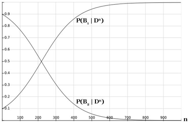
As we can see, our credence in B1 approaches 100% exponentially quickly, and our credence in B2 drops to 0% exponentially quickly. Even if we start with an enormously low prior in B1, our credence will eventually be swamped as we gather more and more data.

It looks like in this example, the Bayesian is successfully hoodwinked by the cheating theory, B1. But this is not quite the end of the story for Bayes. The only single theory that perfectly predicts all of the data you receive in the infinite evidence limit is basically just the theory that “Everything that’s going to happen is what’s going to happen.” And, well, this is surely true. It’s just not very useful.

If instead we look at B1 as a sequence of theories, one for each new data point, then we have a way out by claiming that our priors drop as we go further in the sequence. This is an appeal to simplicity – a theory that exactly specifies 1000 different data points is more complex than a theory that exactly specifies 100 different data points. It also suggests a precise way to formalize simplicity, by encoding it into our priors.

While the problem of over-fitting is not an open-and-shut case against Bayesianism, it should still give us pause. The core of the issue is that there are more intuitive epistemic virtues than those that the Bayesian optimizes for. Bayesianism mandates a degree of belief as a function of two ingredients: the prior and the evidential update. The second of these, Bayesian updating, solely optimizes for accommodation of data. And setting of priors is typically done to optimize for some notion of simplicity. Since empirically distinguishable theories have their priors washed out in the limit of infinite evidence, Bayesianism becomes a primarily accommodating epistemology.

This is what creates the potential for problems of overfitting to arise. The Bayesian is only optimizing for accommodation and simplicity, but what we want is a framework that also optimizes for prediction. I’ll give two examples of ways to do this: cross validation and posterior predictive checking.

I’ve talked about cross validation previously. The basic idea is that you split a set of data into a training set and a testing set, optimize your model for best fit with the training set, and then see how it performs on the testing set. In doing so, you are in essence estimating how well your model will do on predictions of future data points.

This procedure is pretty commonsensical. Want to know how well your model does at predicting data? Well, just look at the predictions it makes and evaluate how accurate they were. It is also completely outside of standard Bayesianism, and solves the issues of overfitting. And since the first half of cross validation is training your model to fit the training set, it is optimizing for both accommodation and prediction.

Posterior predictive checks are also pretty commonsensical; you ask your model to make predictions for future data, and then see how these predictions line up with the data you receive.

More formally, if you have some set of observable variables X and some other set of parameters A that are not directly observable, but that influence the observables, you can express your prior knowledge (before receiving data) as a prior over A, P(A), and a likelihood function P(X | A). Upon receiving some data D about the values of X, you can update your prior over A as follows:

P(A) becomes P(A | D)
where P(A | D) = P(D | A) P(A) / P(D)

To make a prediction about how likely you think it is that the next data point will be X, given the data D, you must use the posterior predictive distribution:

P(X | D) = ∫ P(X | A) ∙ P(A | D) dA

This gives you a precise probability that you can use to evaluate the predictive accuracy of your model.

There’s another goal that we can aim towards, besides accommodation, simplicity, or prediction. This is distance from truth. You might think that this is fairly obvious as a goal, and that all the other methods are really only attempts to measure this. But in information theory, there is a precise way in which you can specify the information gap between any given theory and reality. This metric is called the Kullback-Leibler divergence (DKL), and I’ll refer to it as just information divergence.

DKL = ∫ Ptrue log(Ptrue / P) dx

This term, if parsed correctly, represents precisely how much information you gain if you go from your starting distribution P to the true distribution Ptrue.

For example, if you have a fair coin, then the true distribution is given by (Ptrue(H) = .5, Ptrue(T) = .5). You can calculate how far any other theory (P(H) = p, P(T) = 1 – p) is from the truth using DKL.

 DKL = .5 ∙ [ log(1 / 2p) + log(1 / 2(1-p)) ]

I’ve graphed DKL as a function of p here:

Information divergence.png

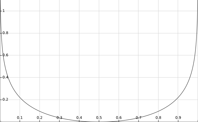
As you can see, the information divergence is 0 for the correct theory that the coin is fair (p = 0.5), and goes to infinity as you get further away from this.

This is all well and good, but how is this practically applicable? It’s easy to minimize the distance from the true distribution if you already know the true distribution, but the problem is exactly that we don’t know the truth and are trying to figure it out.

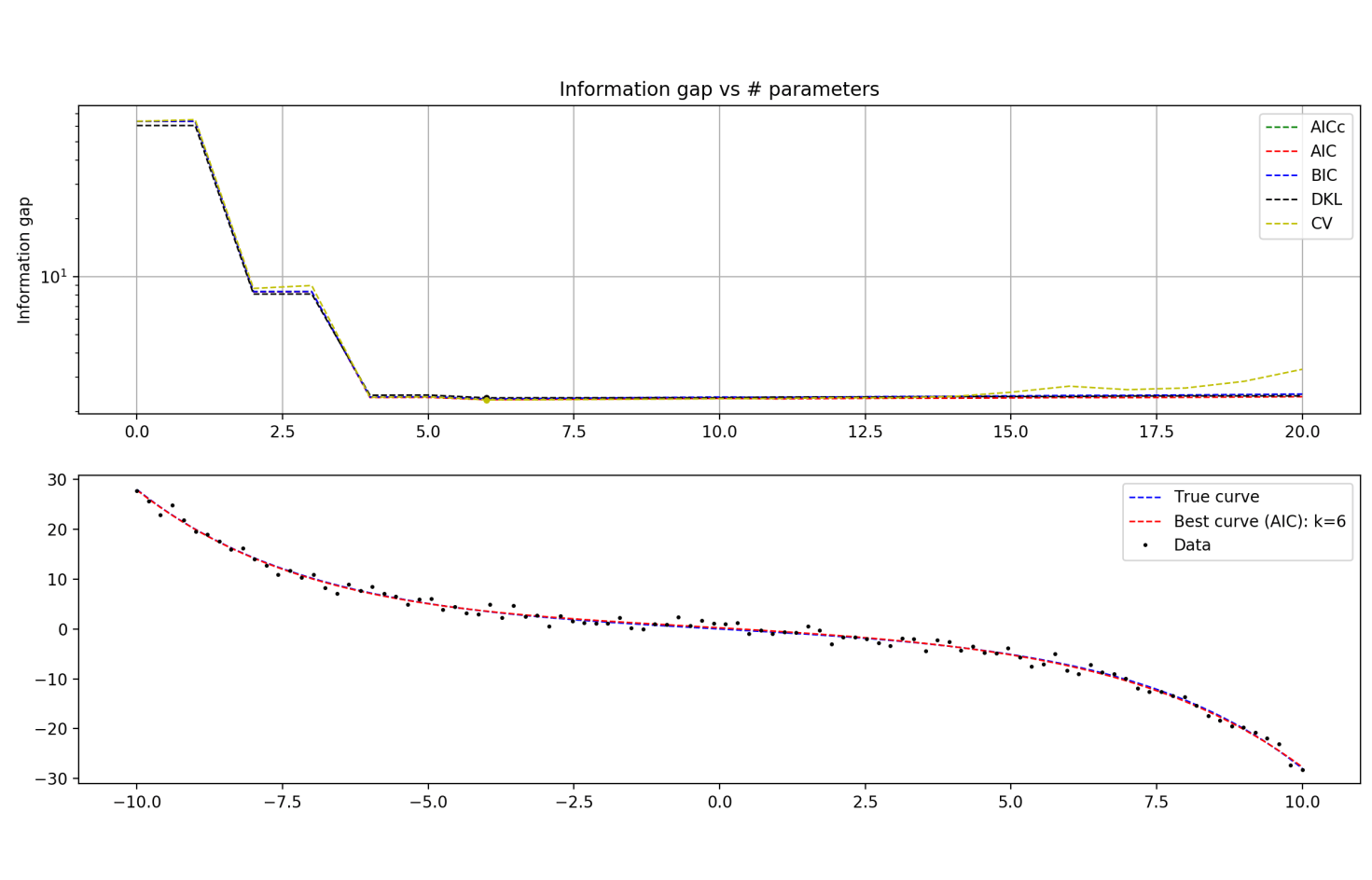
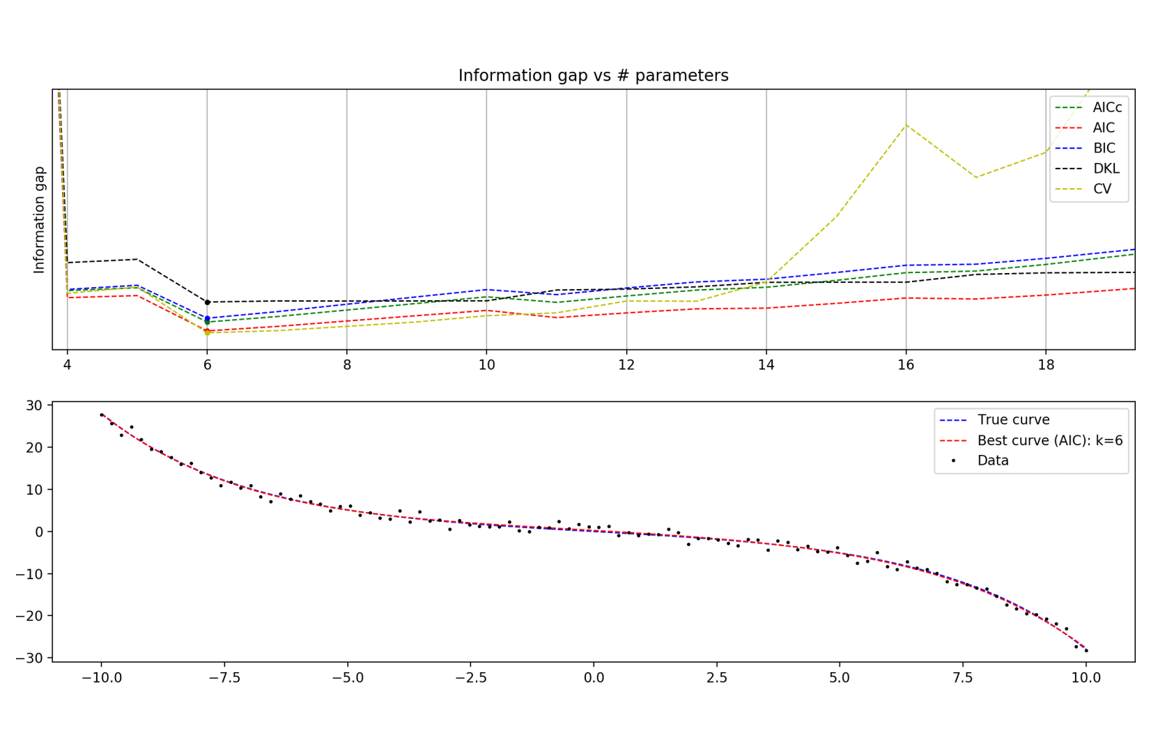
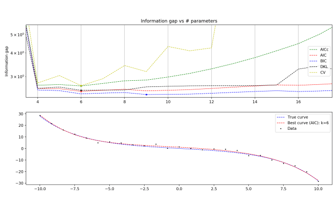
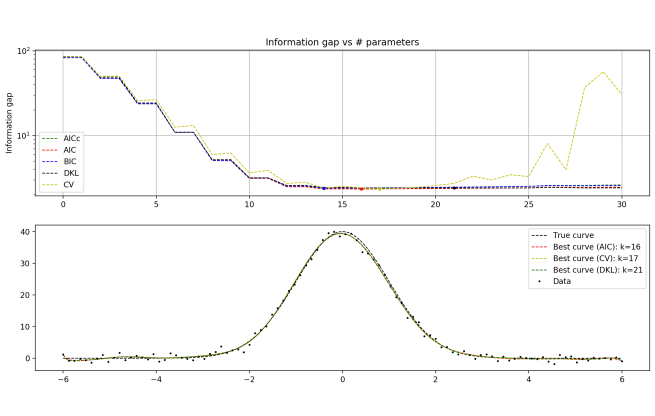
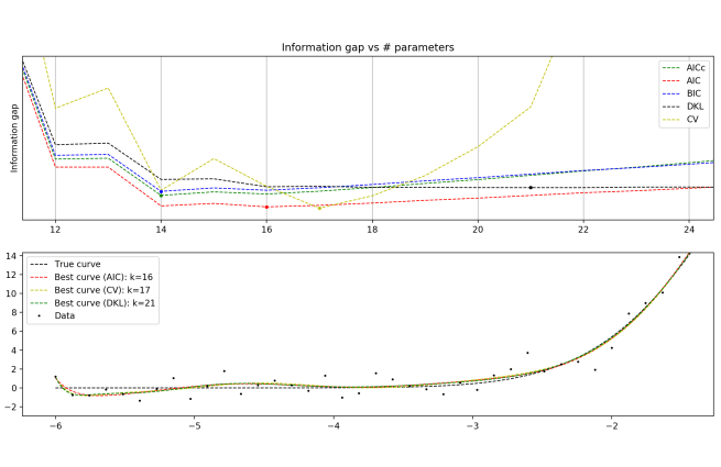
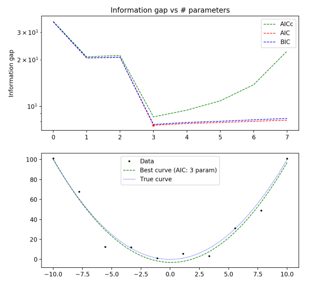
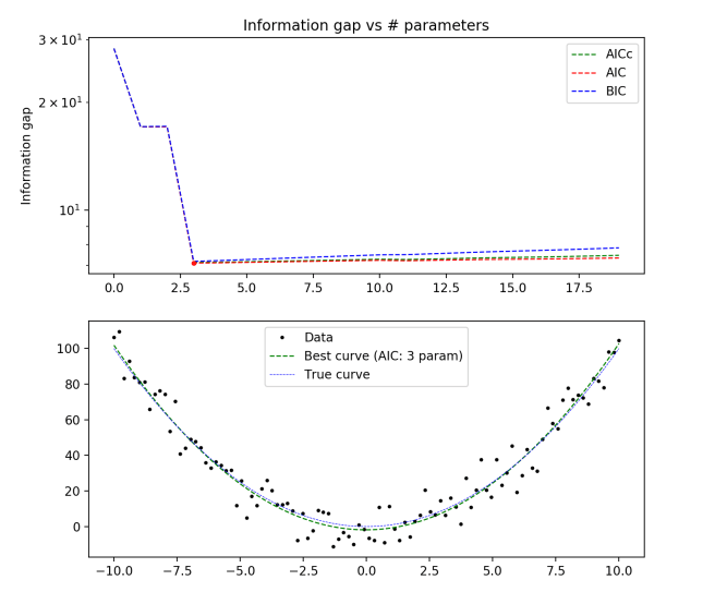
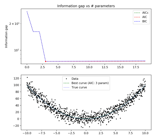
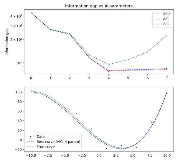
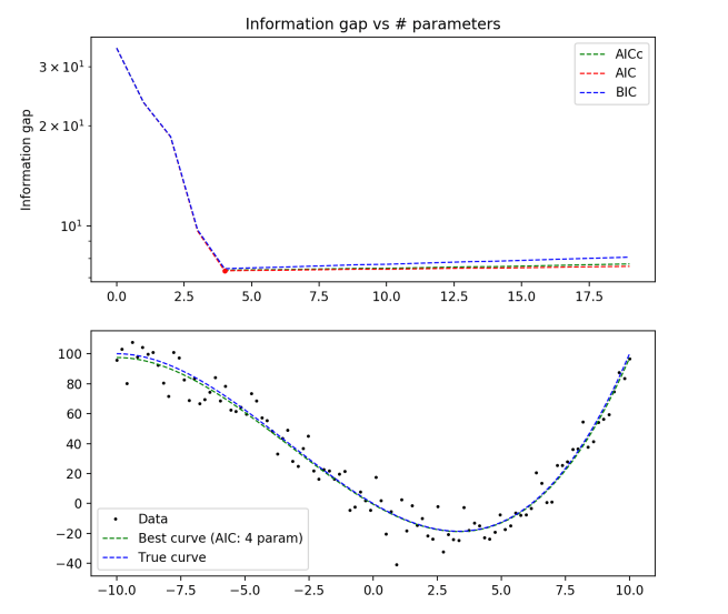
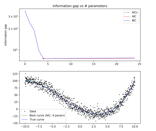
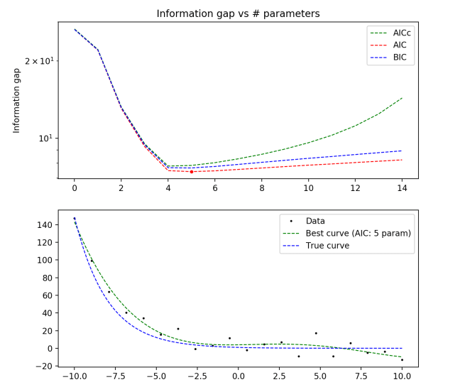
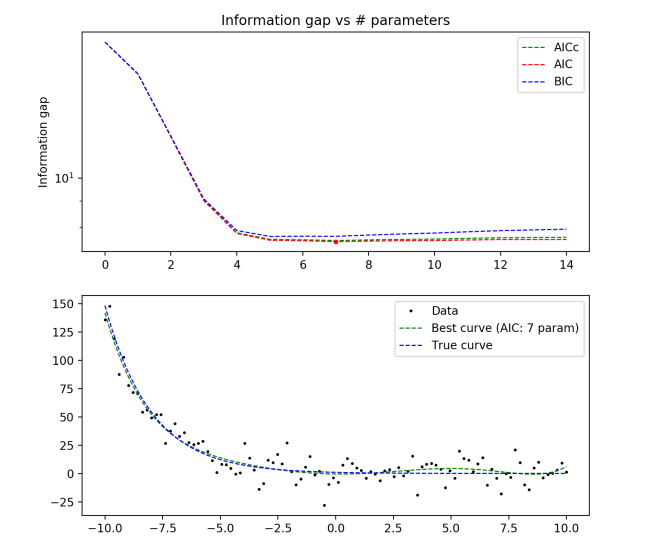
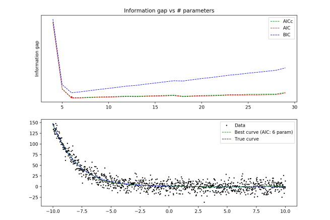
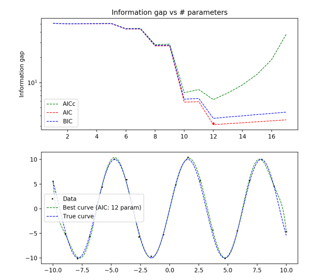
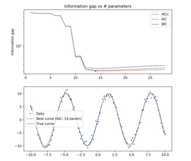
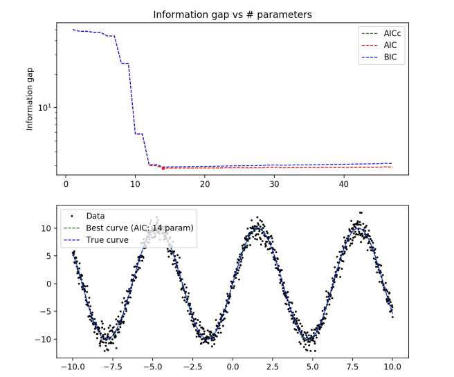
Since we don’t have direct access to Ptrue, we must resort to approximations of DKL. The most famous approximation is called the Akaike information criterion (AIC). I won’t derive the approximation here, but will present the form of this quantity.

AIC = k – log(P(data | M))
where M = the model being evaluated
and k = number of parameters in M

The model that minimizes this quantity probably also minimizes the information distance from truth. Thus, “lower AIC value” serves as a good approximation to “closer to the truth”. Notice that AIC explicitly takes into account simplicity; the quantity k tells you about how complex a model is. This is pretty interesting in it’s own right; it’s not obvious why a method that is solely focused on optimizing for truth will end up explicitly including a term that optimizes for simplicity.

Here’s a summary table describing the methods I’ve talked about here (as well as some others that I haven’t talked about), and what they’re optimizing for.

Goal

Method(s)
Which theory makes the data most likely?

Maximum likelihood estimation (MLE)
p-testing

Which theory is most likely, given the data?

Bayes
Bayesian information criterion (BIC)
Maximum uncertainty

Entropy
Relative entropy

Simplicity

Minimum description length
Solomonoff induction

Predictive accuracy

Cross validation
Posterior predictive checks

Distance from truth

Information divergence (DKL)
Akaike information criterion (AIC)


Racism and identity

I recently saw that a friend of a friend of mine was writing in a blog about her experience as a mixed race woman in America, and all of the ways in which she feels that she suffers from explicit and implicit discrimination. The impression she conveyed was that she walked around intensely aware of her skin color, and felt that others were equally aware. In her world, people looked at her as primarily a brown woman, a strange and exotic other. She talked about the emotional shock she has to go through when returning to the United States after visiting her family in Thailand, in dealing with the fact that Thai culture is so underrepresented here. There was a lot of anger, a feeling of not being accepted by the majority culture around her, and most of all, a sense of being disrespected and harmed on the basis of her ethnicity.

Whenever I hear people like her talking like this, I get really confused. I am a mixed-race person, living in the same city as her, surrounded by probably very similar people, and yet we seem to live in completely different worlds. I know that the idea of color-blindness is not in vogue, but I walk around literally entirely unaware of my skin color and feel fairly confident that almost everybody else I run into is similarly unaware of it.

I’m somebody that’s fairly attuned to social signals – I feel like if I was being slighted on the basis of my ethnicity, I would notice it – and I’m also not somebody that could remotely pass for white. So I’m left wondering… what’s going on here? How can two people have such radically different experiences of living with their ethnicities, when it seems like so many of the variables are the same?

One answer is that some of the variables that appear to be the same actually aren’t. For instance, while we’re both mixed race, we are different mixes of races. While I could pass (and have passed) for Black, Hispanic, Middle Eastern, or Indian, I’ve never been identified as Southeast Asian. So perhaps while Black/Hispanic/Middle Eastern/Indian people face very little racism in my town, Southeast Asians are relentlessly oppressed. Hmm, somehow that seems wrong…

Maybe a relevant difference is the social circles we surround ourselves with. From what I know of this person, she surrounds herself with people that are very concerned with social justice issues. It seems fairly plausible to me that the types of people that are very concerned with social justice are also going to be very sensitive to racial and ethnic identities, and will be much more likely to see somebody as a mixed-race person (and treat this as an important aspect of their identity). Incidentally, the few people who I’ve actually felt conscious of my skin color or ethnicity around have been exactly those people who are most vocal and passionate about their anti-racism and social justice concerns. Also, anecdotally, the people I know who most strongly emphasize feelings of personal oppression happen to surround themselves with social justice types. Of course, this doesn’t indicate the direction of causation – it could be that those that feel oppressed seek out social justice types that will affirm their feelings of being wronged.

Another possibility to explain the difference in perceptions is that one of us is just wrong. Maybe the oppression and constant discrimination and other-ing is actually in my Southeast Asian friend-of-friend’s head. Or maybe I’m actually being horribly oppressed and discriminated against and just don’t know it. Maybe I’m just extremely lucky and have by chance avoided all the nasty racists in my town. (If one of us is wrong, I’m betting it’s her.)

But this isn’t the only time I’ve noticed this disconnect in experiences. I’m reminded of a debate I watched a while back about sexual harassment. The actual debate itself wasn’t too interesting, but I found the Q&A period fascinating. Many different women stood up and spoke about their personal experiences of sexual harassment in their daily life, and what they said completely contradicted each other. Some women claimed that they felt sexually harassed or at risk of sexual harassment virtually always, like, walking in the middle of the day in a public area or shopping for groceries. Other women claimed that they had never been catcalled, nor sexually harassed or discriminated against because of their sex.

Keep in mind; this was a live debate, with a local audience. All of these women lived in the same area. There weren’t obvious differences in their appearances, or ages, or mannerisms, although there were significant differences in their views on sexual harassment (for obvious reasons). Also keep in mind that some of the claims being made were literally just objectively verifiable factual statements. It’s not like the disagreement was over whether others had objectifying thoughts about them because of their sex. The differences were about things like whether or not they are verbally catcalled while walking downtown. There’s got to be an actual fact about how likely the average woman is to be catcalled on a given street.

This is pretty hard to make sense of, and seems like the exact same phenomenon as what’s going on with my friend’s friend and I. People that should be living in similar worlds mentally feel like they are living in completely different worlds.

One last example: I’ve had similar experiences with my sister. She is the same race as me (shocking, I know), with basically the same amount of exposure to the non-American side of our cultural heritage, has lived in the same city as me for most of our lives, and is not too different in age from me. But she talks about a strong sense of feeling discriminated against as a brown woman, and has described experiences of oppression that seem totally foreign to me.

Perhaps a component of all of this can be explained by incentives to exaggerate. This aligns with my sense that those that think they are oppressed hang around with social justice types. A lot of social justice culture seems to be devoted to jockeying for oppression points and finding ways to appear as unprivileged as possible. In a social circle in which one can gain social brownie points by being discriminated against, you would expect a general upwards pressure on the level of exaggeration that the average person uses in describing said discrimination.

I feel like I should stop here to emphasize that I’m not suggesting that there isn’t racial and sexual discrimination in the world. There obviously is. What I’m specifically wondering about is how it is that people in little liberal college towns like mine with fairly similar racial backgrounds can have such radically different perspectives on the factual matter of the actual oppression they face. It’s especially puzzling to me given that I’m a brown person who has, as far as I can tell, never faced significant drawbacks on the basis of it, and is most of the time unaware of my skin color.

I think that this unawareness of my skin color provides a hint for explaining what might be actually going on here. Not only am I generally not aware of my skin color, but I have always felt this way. I think that there is a spectrum of natural self-identification tendencies, and a bias towards attributing perceived affronts to the most salient aspects of your identity. Let me unpack this.

It’s not exactly that I’m unaware that I’m brown (I wouldn’t be surprised if somebody showed me a picture of myself and pointed out my skin color). It’s that my brownness is a nonexistent component of the way I think about myself. As far back as I can remember, the salient features of my sense of self have been things like my way of thinking and my personality. I’ve always identified myself as mostly a mind, not a body. I even remember a few bizarre experiences where I looked in a mirror and was momentarily struck by a surreal sense of disconnect, that I happen to exist within this body that seems so obviously distinct from me.

It is also the case that when I perceive that others dislike me and don’t have any sense of why this may be, I naturally tend to assume that their dislike relates to some aspect of my mental characteristics; maybe they don’t like my style of reasoning, or my sense of humor, or some other aspect of my personality. I will almost never attribute their dislike to some physical characteristics of mine.

I perceive myself as primarily a thinker occupying a body that I don’t strongly identify with. But other people identify much more closely with their physicality (skin color, facial features, body type, sex, et cetera). It seems plausible to me that just as I perceive affronts as having to do with properties of my mind, those for whom race is a salient component of their personal identity will perceive affronts as having to do with racism, those who identify with their sex will be more likely to see them as sexism, and so on.

This idea of a spectrum of self-identification tendencies is fairly satisfying to me as an explanation of this phenomenon of radically different perceptions of the world. Two people that appear to exist in very similar social environments can have radically different perceptions of their social environments, because of differences in how they conceive of themselves and the way that this affects their framing of their interactions with others. These differing tendencies are not restricted to body-versus-mind. Some people strongly identify themselves with a profession, a cultural heritage, or a nation. Others identify with an ideology or a religion. And in general, the parts of your identity that feel most salient to you are those that will prickle most readily at perceived affronts.

This relates to the notion in psychology of internal vs external loci of control. When you fail a job interview, you blame the traffic in the morning, or the interviewer’s bias. If you had gotten the job, you would have happily praised your interviewee skills and charming smile. When your neighbor fails a job interview, you attribute it to their poor interviewee skills. That is, you place the locus of control over the outcome wherever it is convenient.

This is called the fundamental attribution error. With respect to themselves, people attribute positive outcomes to features of their own identity, and negative outcomes to features of the external world. With respect to others, they attribute positive outcomes to the external world and negative outcomes to the person’s character.

If you strongly identify as a mixed person, then you will see events in your world as being all about your mixed race. And if you identify as a mind floating about in a body, then things like your race or sex or attractiveness will seem mostly irrelevant to explaining the events in your life. This suggests a sort of self-perpetuating cycle whereby those that identify as X will perceive the world as centered around X, further entrenching the self-identification as X.