Goodstein sequences are amazingly strange and unintuitive. I want to tell you all their unusual properties up-front, but I also don’t want to spoil the surprise. So let me start by defining the Goodstein sequence of a number.

We start by defining the hereditary base-n representation of a number m. We first write m as a sum of powers of n (e.g. for m = 266 and n = 2, we write 266 = 2⁸ + 2³ + 2¹). Now we write each exponent as a sum of powers of n. (So now we have 266 = 2²³ + 2²⁺¹ + 2¹). And we continue this until all numbers in the representation are ≤ n. For 266, our representation stabilizes at 266 = 2²²⁺¹ + 2²⁺¹ + 2¹.

Now we define G_n(m) as follows: if m = 0, then G_n(m) = 0. Otherwise, G_n(m) is the number produced by replacing every n in the hereditary base-n representation of m by n+1 and subtracting 1. So G₂(266) = G₂(2²²⁺¹ + 2²⁺¹ + 2¹) = 3³³⁺¹ + 3³⁺¹ + 3¹ – 1 ≈ 4.4 × 10³⁸.

Finally, we define the Goodstein sequence for a number n as the following:

a₀ = n
a₁ = G₂(a₀)
a₂ = G₃(a₁)
a₃ = G₄(a₂)
And so on.

Let’s take a small starting number and look at its Goodstein sequence. Suppose we start with 4.

a₀ = 4 = 2²
a₁ = 3³ – 1 = 2⋅3² + 2⋅3 + 2 = 26
a₂ = 2⋅4² + 2⋅4 + 1 = 41
a₃ = 2⋅5² + 2⋅5 = 60
a₄ = 2⋅6² + 2⋅6 – 1 = 2⋅6² + 6 + 5 = 83
a₅ = 2⋅7² + 7 + 4 = 109

Now, notice that the sequence always seems to increase. And this makes sense! After all, each step we take, we increase the base of each exponent by 1 (a big increase in the value) and only subtract 1. Here’s a plot of the first 100 values of the Goodstein sequence of 4:

And for further verification, here are the first million values of the Goodstein sequence of 4:

Looks like exponential growth to me! Which, again, is exactly what you’d expect. In addition, the higher the starting value, the more impressive the exponential growth we see. Here we have the first 100 values of the Goodstein sequence of 6:

Notice how after only 100 steps, we’re already at a value of 5 × 10¹⁰! This type of growth only gets more preposterous for larger starting values. Let’s look at the Goodstein sequence starting with 19.

a₀ = 19
a₁ ≈ 7 × 10¹²
a₂ ≈ 1.3 × 10¹⁵⁴
a₃ ≈ 1.8 × 10²¹⁸⁴
And so on.

We can’t even plot a sequence like this, as it’ll just look like two perpendicular lines:

Alright, so here’s a conjecture that hopefully you’re convinced of: Goodstein sequences are always growing. In fact, let’s conjecture something even weaker: Goodstein sequences never terminate (i.e. never go to zero).

We’re finally ready for our first big reveal! Both of these conjectures are wrong! Not only do some Goodstein sequences terminate, it turns out that EVERY Goodstein sequence eventually terminates!

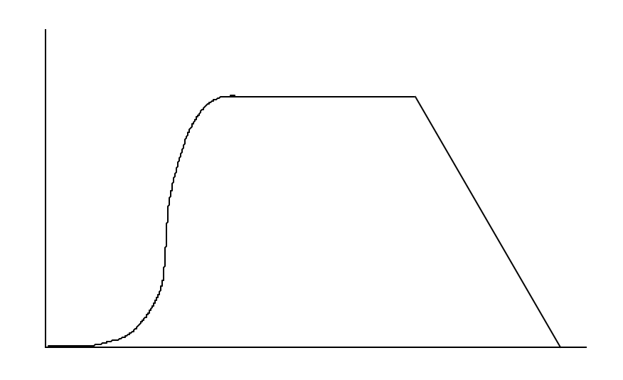
This is pretty mind-blowing. What about all those graphs I showed? Well, the sequences do increase for a very very long time, but they eventually turn around. How long is eventually? The Goodstein sequence of 4 takes 3 × 2^402,653,210 – 1 steps to turn around!! This number is too large for me to be able to actually show you a plot of the sequence turning around. But we do know that once the Goodstein sequence stops increasing, it actually stays fixed for 3 × 2^402,653,209 steps before finally beginning its descent to zero. Heuristically, it would look something like this:

(Why does it stay constant, incidentally? The reason is that when we get to a number whose hereditary base-B notation just looks like B + n for some n < B, we increase B by 1 and decrease n by 1 each step. This doesn’t change the sequence’s value! So it stays constant until we get to n = 0. At that point, we decrease by 1 until we descend all the way to zero.)

So, how do we prove this? We do it using infinite ordinals. (Now you see why this topic caught my eye recently!) The plan is to associate with Goodstein sequence a “matching sequence” of ordinals. The way to do this is pretty simple: for a number written in hereditary base-n notation, just replace every n in that representation with ω. Now you have an infinite ordinal!

So, for example, here’s the first few numbers in the Goodstein sequence of 4, along with their translation to ordinals:

Examine this sequence of ordinals for a couple of minutes. You might notice something interesting: at each step, the ordinal is decreasing! This turns out to always hold true. Let’s see why.

Notice that there are two cases: either the ordinal is a successor ordinal (like ω² + 4), or it’s a limit ordinal (like ω² + ω). If it’s a successor ordinal, then the next ordinal in the sequence is just its predecessor. (So ω² + 4 becomes ω² + 3). This is obviously a smaller ordinal.

What if it’s a limit ordinal? Then the smallest limit ordinal in its expanded representation drops to a smaller limit ordinal and some finite number is added. So for instance, in the ordinal ω² + ω⋅2, ω⋅2 will drop to ω and some finite number will be added on depending on which step in the sequence you’re at. So we’ll end up with ω² + ω + n, for some finite n. This ordinal is smaller than the original one, because we’ve made an infinitely large jump downwards (from one limit ordinal to a lower limit ordinal), and only increased by a finite amount.

So in either case, we go to a smaller ordinal. And now the key realization is that every decreasing sequence of ordinals MUST terminate! (This is one of my favorite facts about ordinals, by the way. Even though we’re looking at arbitrarily large infinite ordinals, it’s still the case that there is no decreasing sequence that goes on forever. Whenever we hit a limit ordinal, we have to make an infinitely large jump downwards to get to the next element in the sequence, as the ordinal has no predecessor.)

So we’ve paired every Goodstein sequence with a decreasing sequence of ordinals. And every decreasing sequence of ordinals eventually terminates. So the Goodstein sequence must terminate as well! (One easy way to see this is to notice that every value in a Goodstein sequence is ≤ the ordinal assigned to it. Another way is to notice that the only number that could possibly be assigned to the ordinal 0 is 0 itself. So when the decreasing sequence of ordinals hits 0, as it must eventually, so must the Goodstein sequence) And that’s our proof!

That Goodstein sequences always terminate is the big flashy result for this post. But there’s much more that’s cool about them. For instance, the proof that we just used did not rely on the fact that we just increased the base by 1 at each step. In fact, even if we update the base by an arbitrarily large function at each stage, the sequences still must terminate!

Even cooler, the proof that all Goodstein sequences terminate cannot be formalized in Peano arithmetic! And in fact, no proof can be found of this theorem using PA. Laurie Kirby and Jeff Paris proved in 1982 that the statement that Goodstein sequences always terminate could be reduced to a theorem of Gentzen from which the consistency of PA could be deduced. So if PA could prove that Goodstein sequences always terminate, then it could prove its own consistency! Gödel’s second incompleteness theorem tells us that this cannot be, and thus assuming that PA really is consistent, it cannot prove that that these sequences all terminate.

This was historically the third result to be found independent of PA, and it was the first that was purely number-theoretic in character (as opposed to meta-mathematical, like the Gödel sentences). It gives us a very salient way of expressing the limitations of Peano arithmetic: simply write a program that computes the Goodstein sequence of any given input, terminating only when it reaches 0 and outputting the length of the sequence. (Code Golf Stack Exchange shows that this can be done using just 77 characters of Haskell! And here’s a nice way to do it in Python). Now, it happens to be true that this program will always terminate for any natural number input (if run on sufficiently powerful hardware). But Peano arithmetic cannot prove this!

As a final fun suprise, let’s define G(n) to be the length of the Goodstein sequence starting at n. As we’ve already seen, this sequence gets really big really quickly. But exactly how quickly does it grow? Turns out that it grows much much faster than other commonly known fast-growing computable functions. For instance, G(n) grows much faster than Ackermann’s function, and G(12) is already greater than Graham’s number!

Peano arithmetic is unable to pin down the natural numbers, despite its countable infinity of axioms. In fact, assuming its consistency Peano arithmetic has models of every cardinality, meaning that as far as PA is aware, there might be uncountably many real numbers. (If PA is not consistent then it has no models.) I want to take a look at these non-standard models of PA, especially the countable ones. A natural question is, how many countable non-standard models are there alongside the standard models?

Assuming the consistency of PA (which I will leave out from now on, as it’s assumed in all that follows), there are continuum many non-isomorphic countable models. That’s a lot! That means that there’s a distinct countable non-standard model of arithmetic for every real number. This is our first result: the number of nonstandard models of PA of cardinality ℵ₀ is 2^ℵ₀. Interestingly, this result generalizes! For every infinite cardinal κ, there are 2^κ non-isomorphic nonstandard models of cardinality κ. That’s a lot of nonstandard models! In fact, since any model of cardinality κ involves a specification of some number of constants, binary relations over κ and functions from κ to κ, we know that the maximum number of models of cardinality κ is 2^κ. So in this sense, Peano arithmetic has as many nonstandard models of each cardinality as it can have!

Let’s take a closer look at the countable non-standard models. It turns out that we can say a lot about their order type. Namely, all countable non standard models of PA have order type ω + (ω*+ω)·η. What does this notation mean? Let me break down each of the order types involved in that formula:

So ω*+ω is the order type of the integer line, and (ω*+ω)·η is the order type of a structure that resembles an integer line for each rational number. Thus, every countable non-standard model of PA looks like a copy of natural numbers followed by as many copies of integers as there are rational numbers. The order on this structure is lexicographic: two nonstandards on the same integer line are judged according to their position on the integer line, and two nonstandards on different integer lines are judged according to the position of these integer lines on the rational line. It’s not the easiest thing to visualize, but here’s my attempt:

So if all countable non-standard models have the same order type, then where do they differ? It turns out that they differ in the details of how addition and multiplication work on the non-standards. (After all, a model of PA is defined by the size of its universe and its interpretation of ≤, +, and ×. Same order type means same ≤, so what’s left to vary is + and ×.) In each of the models, + and × work exactly like normal on the naturals. And + and × must operate on the non-standards in such a way as to maintain the truth of all the axioms of PA. So, for instance, since PA can prove that 2x = x + x, the same must be true for nonstandard x. And so on. But even given these restrictions, there are still uncountably many ways to define + and × on the non-standards.

What’s more, we have a theorem known as the Tennenbaum Theorem, which tells us that it’s impossible to give recursive definitions to + and × in non-standard models. Said more simply, addition and multiplication are uncomputable in every non-standard model of arithmetic!

One thing I remain unsure of is how the nonstandard models of Peano arithmetic compare to the structure of ω in nonstandard models of ZFC. We know that there must be models of ZFC where ω is nonstandard, by the compactness theorem (define ZFC* to be ZFC with an extra constant c, with the extra axioms “c ∈ ω”, “c ≠ 0”, “c ≠ 1”, “c ≠ 2”, and so on. ZFC* has a model by compactness, and this model is also a model of ZFC by monotonicity.) But is ZFC “better” at ruling out nonstandard models of the naturals than PA is? Or is there a nonstandard ω for every nonstandard model of Peano arithmetic?

I want to share a way to construct the order type of the Church-Kleene ordinal ω₁^CK. As far as I’m aware, this construction is original to me, and I think it’s much simpler and more elegant than others that I’ve found on the internet. Please let me know if you see any issues with it!

So, we start with the notion of a computable ordinal. A computable ordinal is a computable well-order on the natural numbers. In other words, it’s a well-order < on ℕ such that there exists a Turing machine that, given any two natural numbers n and m, outputs whether n < m according to that order.

There’s an injection from computable well-orders on ℕ to Turing machines, so there are countably many computable well-orders (at most one for each Turing machine). This means that there’s a list of all such computable well-orders. Let’s label the items on this list in order: {<₀, <₁, <₂, <₃, …}. Each <_n stands for a Turing machine which takes in two natural number inputs and returns true or false based on the nth computable well-ordering.

Now, we want to construct a set with order type ω₁^CK. We’re going to have it be an order on the natural numbers, so what we have to work with from the start is the set {0, 1, 2, 3, 4, 5, 6, …}.

We start by splitting up this set into an infinite collection of sets. First, we take every other number, starting with 0: {0, 2, 4, 6, 8, …}. That’ll be our first set. We’ve left behind {1, 3, 5, 7, 9, …}, so next we take every other number from this set starting with 1: {1, 5, 9, 13, …}. Now we’ve left behind {3, 7, 11, 15, …}. Our next set, predictably, will be every other number from this set starting with 3. This is {3, 11, 19, 27, …}. And we keep on like this forever, until we’ve exhausted every natural number.

This gives us the following set of sets:

{{0, 2, 4, 6, …}, {1, 5, 9, 13, …}, {3, 11, 19, 27, …}, {7, 23, 39, 47, …}, …}

Now, we define our order to make everything in the first set less than everything in the second set, and everything in the second set less than everything in the third set, and so on. So far so good, but this only gives us order type ω². Next we define the order WITHIN each set.

To do this, we’ll use our enumeration of computable orders. In particular, within the nth set, the ith number will be less than the jth number exactly in the case that i <_n j. You can think about this as just treating each set “as if” it’s really {0, 1, 2, 3, …}, then ordering it according to <_n, and then relabeling the numbers back to what they started as.

This fully defines our order. Now, what’s the order type of this set? Well, it can’t be any particular computable order type, because every computable order type can be found as a sub-order of it! So it must be some uncomputable order type. And by construction, we know it must be exactly the order type that contains all and only computable order types as suborders. But this is just the order type of the Church-Kleene ordinal!

So there we have it! We’ve constructed ω₁^CK. Now, remember that the Church-Kleene ordinal is uncomputable. But I just described an apparently well-defined process for creating an ordered set with its order! This means that some part of the process I described must be uncomputable. Challenge question for you: Which part is uncomputable, and can you think of a proof of its uncomputability that is independent of the uncomputability of ω₁^CK?

Take any set and place an order on it. If the order is a well-order (i.e. if every subset has a least element), then the set has the same order type as some particular ordinal. But the notion of order type can be extended beyond well-ordered sets. Any two ordered sets are said to have the same order type if they are order isomorphic: if there’s a bijective map f from one set to the other such that both f and f^-1 preserve the ordering of elements.

One structure that has a very interesting order type is the rational numbers. After all, the rationals are a countable set, but every rational number resembles a “limit ordinal” in the sense that it has no immediate predecessor.

One question that we can ask to get some insight about the order type of the rational numbers is: what ordinals can be found within the rationals? That is, take some well-ordered subset of the rationals. Look at the order type of this subset. This order type corresponds to some ordinal. And different choices of well-ordered subsets of the rationals give us different ordinals! So which ordinals can we “find” within the rationals in this sense?

First off, every finite ordinal can obviously be found. To find the ordinal n, just take the subset {0, 1, 2, …, n-1}. We can also find ω! You can just take the subset {0, 1, 2, 3, …}. What about ω+1? Try for yourself: can you construct a subset of the rationals with the order type of ω+1?

There’s no unique way to do it, but one easy way is to take the subset {1/2, 3/4, 7/8, …, 1}. This set has a countable infinity of elements, one for each natural number, after all of which comes a single element: exactly the order type of ω+1!

If we want a subset of the rationals with order type ω+2, we can use the same trick: {1/2, 3/4, 7/8, …, 1, 2}. And clearly this extends for any ω+n. But how about ω+ω? Can you construct a subset of the rationals with this order type? (Do it yourself before reading on!)

Here’s one way: {1/2, 3/4, 7/8, …, 1+1/2, 1+3/4, 1+7/8, …}. It should be easy to see how to extend this trick to get ω⋅3, ω⋅4, and indeed ω⋅n for any finite n. You can even naturally extend this to get to ω⋅ω. But then what? Are we finished?

If you guessed no, you’re right! We can find subsets of the rationals with order type ω³, and ωⁿ for any finite n, and ω^ω. (Try it!) And we can keep going beyond that as well. So how high can you go?

Turns out that EVERY countable ordinal can be embedded into the rationals, under the usual order! So in some sense the order type of the rationals is as complicated as possible while still being countable. Also, remember that the set of countable ordinals is uncountably large. So this means that the rationals are a countable ordered set that has all of the uncountably many countable ordinals embedded within it! Isn’t that great?

(One thing that makes this seem less insane is that when we’re looking at what ordinals can be embedded in the rationals, we’re searching through different subsets of the rationals. And even though the rationals are countable, the set of all subsets of the rationals is uncountably large.)

One more interesting thing: the set of all subsets of the rationals has cardinality ℶ₁. But the set of all ordinals that can be embedded into the rationals is ω₁, which has cardinality ℵ₁. So if we start with the set of all subsets of the rationals, then strip away all but those that are well-ordered, and then choose just a single representative for each order type, we get a set of cardinality ℵ₁. And there is no guarantee that this final set has the same cardinality as the original set, because this is the continuum hypothesis! This is a way to think about how to “construct” a real life set with cardinality ℵ₁: look at the set of well-ordered subsets of the rationals, and split it into order-type equivalence classes.

One can live without knowing the ordinals, to be sure, but not as well.

Quote from this paper

What is an ordinal number? If you read my previous post, you might be convinced that an ordinal number is a particular type of set that contains all the ordinal numbers less than it. In particular, the ordinal 0 is the empty set, the ordinal 1 is the set {0}, the ordinal 2 is the set {0,1}, and so on. This is a fine way to think about ordinals, but there’s a much deeper view of them that I want to present in this post.

The fundamental concept is that of order types. Order types are to order-preserving bijections as cardinalities are to bijections. If you’ve seen pictures like these before, then they’re good to have in mind when you think about what order types are:

Let’s get into more detail about order types.

Take any two sets. If there is a bijection between them, then we say that they have the same cardinality. So we can think of each cardinal number as a class of sets, all in bijective correspondence with one another.

Take any two well-ordered sets. (Recall, a set is well-ordered if each of its subsets has a least element.) If there is an order-preserving bijection between them, then we say that the two sets have the same order type. So we can think of each ordinal number as a class of sets, all of the same order type.

For instance, the cardinal number “2” is the class of all sets with two elements (as all such sets are in bijective correspondence with one another). And the ordinal number “2” is the class of all well-ordered two-element sets. In particular, Von Neumann’s ordinal 2 = {0, 1} = {∅, {∅}} has this order type.

The finite cardinalities and finite order types line up nicely: any two well-ordered sets with the same finite cardinality are guaranteed to have the same order type. It’s in the realm of the infinite where order types and cardinalities come apart.

The cardinal number ℵ₀ is the class of all sets that can be put into bijective correspondence with the set of natural numbers ω. This includes the set of even numbers and the set of rational numbers. So how many order types are there of sets with cardinality ℵ₀?

Consider the following two ordered sets: X = {0 < 1 < 2 < 3 < …} and Y = {1 < 2 < 3 < … < 0}. They both have cardinality ℵ₀, but do they have the same order types? If so, then there must be a bijection f: X → Y such that f is order-preserving (for all a ∈ X and b ∈ X, if a < b then f(a) < f(b)). But what element of X is mapped to 0 in Y? In the set Y, 0 is larger than every element besides itself, but there is no element of X that has this property! So no, X and Y do not have the same order types.

X is the order type of ω (a countably infinite list of elements with no elements that have infinitely many predecessors), and Y is the order type of ω+1 (a countably infinite list of elements with a single element coming after all of them). This tells us that there are at least two different order types within the cardinality ℵ₀.

Can we construct an order on the set of natural numbers that has the same order type as ω+2? Well, all we need is for there to be two elements that are larger than all the rest. So we can write something like {2 < 3 < 4 < … < 0 < 1}. This generalizes easily to ω+n, for any finite n: {n+1 < n+2 < … < 0 < 1 < … < n} has the same order type as ω+n.

But now what about ω+ω, i.e. ω⋅2? To get a set of naturals with the same order type, we have to use a new trick. We need two countably infinite sequences of numbers that we can place beside one another. An easy way to accomplish this is by using the evens and odds: {0 < 2 < 4 < … < 1 < 3 < 5 < …}.

We can get an order on the naturals with the same order type as ω⋅2 + 1 by just choosing a single natural number to place after all the others. For instance: {2 < 4 < 6 < … < 1 < 3 < 5 < … < 0}. It should be easy to see how to get ω⋅2 + n for any finite n: just do {n < n+2 < n+4 < … < n+1 < n+3 < n+5 < … < 0 < 1 < 2 < … < n-1} And now how about ω⋅3?

(Try it out for yourself before reading on!)

To get ω⋅3, we need to place three countably infinite sequences of naturals side by side. For instance: {0 < 3 < 6 < … < 1 < 4 < 7 < … < 2 < 5 < 8 < …}.

For ω⋅4, we can use a similar trick: {0 < 4 < 8 < … < 1 < 5 < 9 < … < 2 < 6 < 10 < … < 3 < 7 < 11 < …}. Again, we can quite easily generalize this to ω⋅n for any finite n: {0 < n < 2n < … < 1 < n+1 < 2n+1 < … < 2 < n+2 < 2n+2 < … < … < n-1 < 2n-1 < 3n-1 < …}. But how about ω⋅ω? How do we deal with ω²?

This is a fun exercise to try for yourself at home. Construct an order on the set of natural numbers that has the same order type as ω². Then try to generalize the trick to get ω³, ω⁴, and ωⁿ for any finite n.

Next construct an order on the naturals with the same order type as ω^ω! Can you do it for ω^ω^ω? And ω^ω^ω^…? One thing that should become clear is that the larger an ordinal you’re dealing with, the harder it becomes to construct an order on the naturals with the same order type. The natural question is: is it always possible to do this type of construction, or do we at some point run out of clever tricks to use to get to higher and higher countable ordinals?

Well, if an ordinal α is countable, then it is a well-ordered set with the same cardinality as the naturals. So there always exists some order that can be placed on the naturals to mimic the order type of α. But is this order always computable?

We call an order on the naturals computable if there’s some Turing machine which takes as input two naturals x and y and outputs whether x < y according to this order. We call an order type computable if there’s some computable order on the naturals with that order type. The standard order (0 < 1 < 2 < 3 < …) is computable, and it’s easy to see how to compute all the other orders we’ve discussed so far. But are ALL the countable order types computable?

The wonderful and strange answer is no. There are countable order types that are uncomputable! There must exist orders on the naturals with such order types, but these orders are so immensely complicated and strange that they cannot be defined by ANY Turing machine! Here’s a quick and easy proof of this. (The next three paragraphs are the coolest and most important part of this whole post, so pay attention!)

Turn your mind back to Von Neumann’s construction of the ordinals, according to which each ordinal was exactly the set of all smaller ordinals. More technically, a set α is a Von Neumann ordinal iff α is well ordered with respect to ∈ AND every element of α is also a subset of α. Consider now the set of all countable ordinals. It can be seen that this set is itself an ordinal. Can it be a countable ordinal? No, because if it were then it would have to be an element of itself! (This is not allowed in ZFC by the axiom of regularity.) This means that there are uncountably many countable ordinals.

Ok, so far so good. Now we just observe that there are only countably many Turing machines. So there are only countably many Turing machines that compute orders on the naturals. And therefore there are only countably many computable ordinals.

Putting this together, we see that there are uncountably many uncomputable countable order types (say that sentence out loud). After all, there are uncountably many countable ordinals, and only countably many computable ordinals!

And if there’s only countably many computable ordinals, then there’s some countable Von Neumann ordinal consisting of the set of all computable ordinals! This set couldn’t possibly be computable, because then it would be contained within itself. So it’s the smallest uncomputable ordinal! This set is called the Church-Kleene ordinal. Its order type is literally so convoluted and complex that no Turing machine can compute it!