Suppose you have some old distribution Pold, and you want to update it to a new distribution Pnew given some information.
You want to do this in such a way as to be as uncertain as possible, given your evidence. One strategy for achieving this is to maximize the difference in entropy between your new distribution and your old one.
Entropy is expected surprise. So this quantity is the new expected surprise minus the old expected surprise. Maximizing this corresponds to trying to be as much more surprised on average as possible than you expected to be previously.
But this is not quite right. We are comparing the degree of surprise you expect to have now to the degree of surprise you expected to have previously, based on your old distribution. But in general, your new distribution may contain important information as to how surprised you should have expected to be.
Think about it this way.
One minute ago, you had some set of beliefs about the world. This set of beliefs carried with it some degree of expected surprise. This expected surprise is not the same as the true average surprise, because you could be very wrong in your beliefs. That is, you might be very confident in your beliefs (i.e. have very low EXPECTED surprise), but turn out to be very wrong (i.e. have very high ACTUAL average surprise).
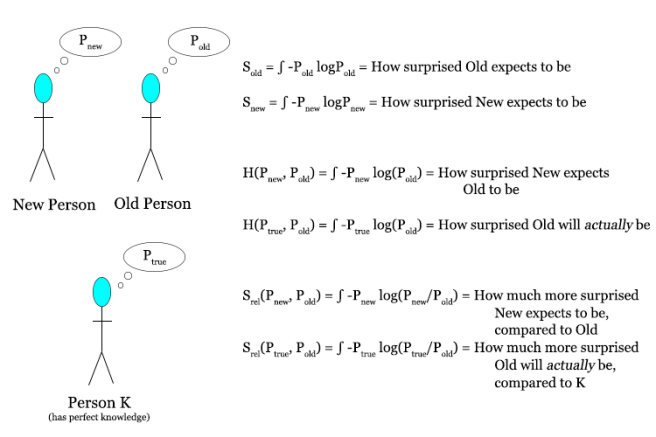
What we care about is not how surprised somebody with the distribution Pold would have expected to be, but how surprised you now expect somebody with the distribution Pold to be. That is, you care about the average value of surprise, given your new distribution, your new best estimate of the actual distribution
That is to say, instead of using the simple difference in entropies S(Pnew) – S(Pold), you should be using the relative entropy Srel(Pnew, Pold).
Max Srel = ∑ -Pnew logPnew – ∑ -Pnew logPold
Here’s a diagram describing the three species of entropy: entropy, cross entropy, and relative entropy.
As one more example of why this makes sense: imagine that one minute ago you were totally ignorant and knew absolutely nothing about the world, but were for some reason very irrationally confident about your beliefs. Now you are suddenly intervened upon by an omniscient Oracle that tells you with perfect accuracy exactly what is truly going on.
If your new beliefs are designed by maximizing the absolute gain in entropy, then you will be misled by your old irrational confidence; your old expected surprise will be much lower than it should have been. If you use relative entropy, then you will be using your best measure of the actual average surprise for your old beliefs, which might have been very large. So in this scenario, relative entropy is a much better measure of your actual change in average surprise than the absolute entropy difference, as it avoids being misled by previous irrationality.
A good way to put this is that relative entropy is better because it uses your current best information to estimate the difference in average surprise. While maximizing absolute entropy differences will give you the biggest change in expected surprise, maximizing relative entropy differences will do a better job at giving you the biggest difference in *actual* surprise. Relative entropy, in other words, allows you to correct for previous bad estimates of your average surprise, and substitute in the best estimate you currently have.
These two approaches, maximizing absolute entropy difference and maximizing relative entropy, can give very different answers for what you should believe. It so happens that the answers you get by maximizing relative entropy line up nicely with the answers you get from just ordinary Bayesian updating, while the answers you get by maximizing absolute entropy differences, which is why this difference is important.
This post is for anybody that is confused about the numerous different types of entropy concepts out there, and how they relate to one another. The concepts covered are:
Surprise
Information
Entropy
Cross entropy
KL divergence
Relative entropy
Log loss
Akaike Information Criterion
Cross validation
Let’s dive in!
Surprise and information
Previously, I talked about the relationship between surprise and information. It is expressed by the following equation:
Surprise = Information = – log(P)
I won’t rehash the justification for this equation, but highly recommend you check out the previous post if this seems unusual to you.
In addition, we introduced the ideas of expected surprise and total expected surprise, which were expressed by the following equations:
Expected surprise = – P log(P) Total expected surprise = – ∑ P log(P)
As we saw previously, the total expected surprise for a distribution is synonymous with the entropy of somebody with that distribution.
Which leads us straight into the topic of this post!
Entropy
The entropy of a distribution is how surprised we expect to be if we suddenly learn the truth about the distribution. It is also the amount of information we expect to gain upon learning the truth.
A small degree of entropy means that we expect to learn very little when we hear the truth. A large degree of entropy means that we expect to gain a lot of information upon hearing the truth. Therefore a large degree of entropy represents a large degree of uncertainty. Entropy is our distance from certainty.
Entropy = Total expected surprise = – ∑ P log(P)
Notice that this is not the distance from truth. We can be very certain, and very wrong. In this case, our entropy will be high, because it is our expected surprise. That is, we calculate entropy by looking at the average surprise over our probability distribution, not the true distribution. If we want to evaluate the distance from truth, we need to evaluate the average over the true distribution.
We can do this by using cross-entropy.
Cross Entropy
In general, the cross entropy is a function of two distributions P and Q. The cross entropy of P and Q is the surprise you expect somebody with the distribution Q to have, if you have distribution P.
Cross Entropy = Surprise P expects of Q = – ∑ P log(Q)
The actual average surprise of your distribution P is therefore the cross-entropy between P and the true distribution. It is how surprised somebody would expect you to be, if they had perfect knowledge of the true distribution.
Actual average surprise = – ∑ Ptrue log(P)
Notice that the smallest possible value that the cross entropy could take on is the entropy of the true distribution. This makes sense – if your distribution is as close to the truth as possible, but the truth itself contains some amount of uncertainty (for example, a fundamentally stochastic process), then the best possible state of belief you could have would be exactly as uncertain as the true distribution is. Maximum cross entropy between your distribution and the true distribution corresponds to maximum distance from the truth.
Kullback-Leibler divergence
If we want a quantity that is zero when your distribution is equal to the true distribution, then you can shift the cross entropy H(Ptrue, P) over by the value of the true entropy S(Ptrue). This new quantity H(Ptrue, P) – S(Ptrue) is known as the Kullback-Leibler divergence.
Shifted actual average surprise = Kullback-Leibler divergence = – ∑ Ptrue log(P) + ∑ Ptrue log(Ptrue) = ∑ Ptrue log(Ptrue/P)
It represents the information gap, or the actual average difference in difference between your distribution and the true distribution. The smallest possible value of the Kullback-Leibler divergence is zero, when your beliefs are completely aligned with reality.
Since KL divergence is just a constant shift away from cross entropy, minimizing one is the same as minimizing the other. This makes sense; the only real difference between the two is whether we want our measure of “perfect accuracy” to start at zero (KL divergence) or to start at the entropy of the true distribution (cross entropy).
Relative Entropy
The negative KL divergence is just a special case of what’s called relative entropy. The relative entropy of P and Q is just the negative cross entropy of P and Q, shifted so that it is zero when P = Q.
Since the cross entropy between P and Q measures how surprised P expects Q to be, the relative entropy measures P’s expected gap in average surprisal between themselves and Q.
KL divergence is what you get if you substitute in Ptrue for P. Thus it is the expected gap in average surprisal between a distribution and the true distribution.
Applications
Maximum KL divergence corresponds to maximum distance from the truth, while maximum entropy corresponds to maximum from certainty. This is why we maximize entropy, but minimize KL divergence. The first is about humility – being as uncertain as possible given the information that you possess. The second is about closeness to truth.
Since KL divergence is just a constant shift away from cross entropy, minimizing one is the same as minimizing the other. This makes sense, the only real difference between the two is whether we want our “perfectly accurate” measure to start at zero (KL divergence) or at the entropy of the true distribution (cross entropy).
Since we don’t start off with access to Ptrue, we can’t directly calculate the cross entropy H(Ptrue, P). But lucky for us, a bunch of useful approximations are available!
Log loss
Log loss uses the fact that if we have a set of data D generated by the true distribution, the expected value of F(x) taken over the true distribution will be approximately just the average value of F(x), for x in D.
Cross Entropy = – ∑ Ptrue log(P) (Data set D, N data points)
Cross Entropy ~ Log loss = – ∑x in D log(P(x)) / N
This approximation should get better as our data set gets larger. Log loss is thus just a large-numbers approximation of the actual expected surprise.
Akaike information criterion
Often we want to use our data set D to optimize our distribution P with respect to some set of parameters. If we do this, then the log loss estimate is biased. Why? Because we use the data in two places: first to optimize our distribution P, and second to evaluate the information distance between P and the true distribution.
This allows problems of overfitting to creep in. A distribution can appear to have a fantastically low information distance to the truth, but actually just be “cheating” by ensuring success on the existing data points.
The Akaike information criterion provides a tweak to the log loss formula to try to fix this. It notes that the difference between the cross entropy and the log loss is approximately proportional to the number of parameters you tweaked divided by the total size of the data set: k/N.
Thus instead of log loss, we can do better at minimizing cross entropy by minimizing the following equation:
AIC = Log loss + k/N
(The exact form of the AIC differs by multiplicative constants in different presentations, which ultimately is unimportant if we are just using it to choose an optimal distribution)
The explicit inclusion of k, the number of parameters in your model, represents an explicit optimization for simplicity.
Cross Validation
The derivation of AIC relies on a complicated set of assumptions about the underlying distribution. These assumptions limit the validity of AIC as an approximation to cross entropy / KL divergence.
But there exists a different set of techniques that rely on no assumptions besides those used in the log loss approximation (the law of large numbers and the assumption that your data is an unbiased sampling of the true distribution). Enter the holy grail of model selection!
The problem, recall, was that we used the same data twice, allowing us to “cheat” by overfitting. First we used it to tweak our model, and second we used it to evaluate our model’s cross entropy.
Cross validation solves this problem by just separating the data into two sets, the training set and the testing set. The training set is used for tweaking your model, and the testing set is used for evaluating the cross entropy. Different procedures for breaking up the data result in different flavors of cross-validation.
There we go! These are some of the most important concepts built off of entropy and variants of entropy.
Today we’re going to talk about a topic that’s very close to my heart: entropy. We’ll start somewhere that might seem unrelated: surprise.
Suppose that we wanted to quantify the intuitive notion of surprise. How should we do that?
We’ll start by analyzing a few base cases.
First! If something happens and you already were completely certain that it would happen, then you should completely unsurprised.
That is, if event E happens, and you had a credence P(E) = 100% in it happening, then your surprise S should be zero.
S(1) = 0
Second! If something happens that you were totally sure was impossible, with 100% credence, then you should be infinitely surprised.
That is, if E happens and P(E) = 0, then S = ∞.
S(0) = ∞
So far, it looks like your surprise S should be a function of your credence P in the event you are surprised at. That is, S = S(P). We also have the constraints that S(1) = 0 and S(0) = ∞.
There are many candidates for a function like this, for example: S(P) = 1/P – 1, S(P) = -log(P), S(P) = cot(πx/2). So we need more constraints.
Third! If an event E1 happens that is surprising to degree S1, and then another event E2 happens with surprisingness S2, then your surprise at the combination of these events should be S1 + S2.
I.e., we want surprise to be additive. If S(P(E1)) = S1 and S(P(E2 | E1)) = S2, then S(P(E1 & E2) = S1 + S2.
This entails a new constraint on our surprise function, namely:
S(PQ) = S(P) + S(Q)
Fourth, and finally! We want our surprise function to be continuous – free from discontinuous jumps. If your credence that the event will happen changes by an arbitrarily small amount, then your surprise if it does happen should also change by an arbitrarily small amount.
S(P) is continuous.
These four constraints now fully specify the form of our surprise function, up to a multiplicative constant. What we find is that the only function satisfying these constraints is the logarithm:
S(P) = k logP, where k is some negative number
Taking the simplest choice of k, we end up with a unique formalization of the intuitive notion of surprise:
S(P) = – logP
To summarize what we have so far: Four basic desideratum for our formalization of the intuitive notion of surprise have led us to a single simple equation.
This equation that we’ve arrived at turns out to be extremely important in information theory. It is, in fact, just the definition of the amount of information you gain by observing E. This reveals to us a deep connection between surprise and information. They are in an important sense expressing the same basic idea: more surprising events give you more information, and unsurprising events give you little information.
Let’s get a little better numerical sense of this formalization of surprise/information. What does a single unit of surprise or information mean? With some quick calculation, we see that a single unit of surprise, or bit of information corresponds to the observation of an event that you had a 50% expectation of. This also corresponds to a ruling out of 50% of the weight of possible other events you thought you might have observed. In essence, each bit of information you receive / surprise you experience corresponds to the total amount of possibilities being cut in half.
Two bits of information narrow the possibilities to one-fourth. Three cut out all but one-eighth. And so on. For a rational agent, the process of receiving more information or of being continuously surprised is the process of whittling down your models of reality to a smaller and better set!
The next great step forward is to use our formalization of surprise to talk not just about how surprised you are once an event happens, but how surprised you expectto be. If you have a credence of P in an event happening, then you expect a degree of surprise S(P) with credence P. In other words, the expected surprise you have with respect to that particular event is:
Expected surprise = – P logP
When summed over the totality of all possible events that occurred we get the following expression:
Total expected surprise = – ∑i Pi logPi
This expression should look very very familiar to you. It’s one of the most important quantities humans have discovered…
ENTROPY!!
Now you understand the title of this post. Quite literally, entropy is total expected surprise!
Entropy = Total expected surprise
By the way, you might be wondering if this is the same entropy as you hear mentioned in the context of physics (that thing that always increases). Yes, it is identical! This means that we can describe the Second Law of Thermodynamics as a conspiracy by the universe to always be as surprising as possible to us! There are a bunch of ways to explore the exact implications of this, but that’s a subject for another post.
Getting back to the subject of this post, we can now make another connection. Surprise is information. Total expected surprise is entropy. And entropy is a measure of uncertainty.
If you think about this for a moment, this should start to make sense. If your model of reality is one in which you expect to be very surprised in the next moment, then you are very uncertain about what is going to happen in the next moment. If, on the other hand, your model of reality is one in which you expect zero surprise in the next moment, then you are completely certain!
Thus we see the beautiful and deep connection between surprise, information, entropy, and uncertainty. The overlap of these four concepts is rich with potential for exploration. We could go the route of model selection and discuss notions like mutual information, information divergence, and relative entropy, and how they relate to the virtues of predictive accuracy and model simplicity. We could also go the route of epistemology and discuss the notion of epistemic humility, choosing your beliefs to maximize your uncertainty, and the connection to Bayesian epistemology. Or, most tantalizingly, we could go the route of physics and explore the connection between this highly subjective sense of entropy as surprise/ uncertainty, and the very concrete notion of entropy as a physical quantity that characterizes the thermal properties of systems.
Instead of doing any of these, I’ll do none, and end here in hope that I’ve conveyed some of the coolness of this intersection of philosophy, statistics, and information theory.
I like to try to surround myself with people that are very intelligent and know a lot about subjects that I know very little about. As such, I am sometimes in the position that Scott Alexander refers to as epistemic learned helplessness. The basic idea bears some resemblance to ideas I explored in a previous post about reasoning in the presence of Super Persuaders.
When you’re talking to somebody who is much more knowledgeable than you about a particular subject and who is presenting to you very compelling arguments, it becomes unclear how strongly you should update on the arguments you are receiving. In particular, if the person you’re talking to is very plausibly presenting a biased sampling of the relevant arguments, then you should be very hesitant to update on these arguments as fully as you would otherwise.
One way of dealing with this is just to avoid people that know more than you and have strong opinions on matters that are disputed among experts. But that’s no fun.
A useful heuristic here is to do your best to imagine what it would be like if there was a rival expert in the room with you and your conversation partner. Creatively, I call this the Rival-Expert Heuristic.
For example, imagine that you’re in conversation with an expert sociologist who is making some very compelling-sounding arguments for why socialist economic systems are overall better than capitalistic systems. It might be that you can’t personally see any reason why the arguments they’re making would fail, and are unable to think of any original arguments for capitalism or against socialism.
In such a situation, it might be genuinely helpful to imagine that Milton Friedman is sitting in the room beside you, holding forth against the scholar. Even if you don’t personally know any counterarguments, you might have some sense that it is likely that such counterarguments exist and that Milton Friedman would know them.
If they say “Capitalism is a system that exploits workers and causes wealth to concentration at the top!”, and you don’t know of any good responses to this, you should consider the chance that Milton Friedman has heard of this line of argument and has a crushingly good response to it. If you can’t think of arguments of your own to present, you should try to take into account the “empty space” in the conversation where these opposing arguments would be if Milton Friedman was in the room.
This can potentially help you with judging how strong the arguments you’re receiving actually are. The primary difficulty is obvious: it’s not easy to accurately imagine a rival expert for exactly the reason that you don’t personally know what arguments they would be making.
At the same time, it is probably much easier to simply consider the question: “How likely is it that a rival expert would have a compelling response to this?” than it is to try to construct such a response yourself. I also think that it can be more reliable in many cases. Imagine that somebody comes up to you with plans for a perpetual motion device, and begins to describe them in much greater detail than you are able to understand. Perhaps this person understands the underlying physics much better than you, and whenever you raise an objection to their design, they are able to easily respond with apparently logical arguments. This is a case where you can be extremely confident that there exist good reasons why they are wrong, even though you have no idea what those reasons might be.
More realistically, suppose that somebody presents you with an argument for why X is true, and you vividly remember hearing a fantastic argument just last week for the falsity of X by a very reputable expert on X-like matters. The trouble is, you can’t remember any of the details of this argument, just that it was a much stronger argument by a more reputable source that this argument you are receiving now. This is a situation that we are often in, but is not typically addressed in standard philosophy talk about epistemology.
Are we justified in believing that what they’re saying is probably wrong, even though we can’t remember the details of the argument? Of course! Our confidence in the falsity of X is moved by an argument’s strength, only indirectly by its content. If the memory of the strength of the argument is retained and reliable, then there is no reason to backtrack on the earlier credence bump.
But just feeling confident that the things you’re hearing are wrong is often not very salient to us, especially if the person saying them is very charismatic and persuasive. You’ll eventually be tempted to relent in your dogged agnosticism after repeatedly failing to see any flaws in their arguments.
This, I think, is the main strength of the rival-expert heuristic. Dogged adherence to uncertainty in the face of compelling evidence feels much more okay if you can vividly imagine a more balanced social dynamic, one in which compelling evidence is being presented on both sides of the issue.
A more general form of this heuristic is to not form strong opinions or take sides on issues that are controversial amongst those that know the most on them, unless you yourself are one of the top experts. I think that a world in which this was more common would be hugely improved. As it is, people generally have far too many beliefs that are far too strong on matters that are disputed among experts. Part of the problem is that beliefs are sticky – It’s easier to acquire them than it is to abandon them once they have become a part of your identity.
If you think that raising the minimum wage is obviously a fantastic idea, but also know that there is a great deal of complicated debate amongst professional economists on the matter, then you are implicitly assuming that you know better than all those economists that disagree with you.
More viscerally, you must come to terms with the fact that if you were faced with the boatloads of experts that disagree with you, your arguments would probably fall flat, and you would likely hear a bunch of compelling arguments for why you are wrong. If this is true, then you essentially are just hanging on to your beliefs because you have by chance happened to avoid these experts!
Ultimately, the Rival-Expert Heuristic is about updating on evidence that you don’t have, but which you have good reason to believe exists. Perhaps this feels weird, but to sum up, there are three basic motivations for doing so.
First, we are easily convinced by compelling-sounding arguments from biased sources.
Second, abstractly knowing of the existence of experts that disagree with compelling-sounding arguments is less likely to properly influence your epistemic habits than actually imagining those experts engaging with the arguments.
And third, beliefs are “sticky” and easier to take on than to back out of.
(This post is a soft intro to some of the many interesting aspects of model selection. I will inevitably skim over many nuances and leave out important details, but hopefully the final product is worth reading as a dive into the topic. A lot of the general framing I present here is picked up from Malcolm Forster’s writings.)
What is the optimal algorithm for discovering the truth? There are many different candidates out there, and it’s not totally clear how to adjudicate between them. One issue is that it is not obvious exactly how to measure correspondence to truth. There are several different criterion that we can use, and in this post, I want to talk about three big ones: accommodation, prediction, and simplicity.
The basic idea of accommodation is that we want our theories to do a good job at explaining the data that we have observed. Prediction is about doing well at predicting future data. Simplicity is, well, just exactly what it sounds like. Its value has been recognized in the form of Occam’s razor, or the law of parsimony, although it is famously difficult to formalize.
Let’s say that we want to model the relationship between the number of times we toss a fair coin and the number of times that it lands H. We might get a data set that looks something like this:
Now, our goal is to fit a curve to this data. How best to do this?
Consider the following two potential curves:
Curve 1 is generated by Procedure 1: Find the lowest-order polynomial that perfectly matches the data.
Curve 2 is generated by Procedure 2: Find the straight line that best fits the data.
If we only cared about accommodation, then we’ll prefer Curve 1 over Curve 2. After all, Curve 1 matches our data perfectly! Curve 2, on the other hand, is always close but never exactly right.
On the other hand, regardless of how well Curve 1 fits the data, it entirely misses the underlying pattern in the data captured by Curve 2! This demonstrates one of the failure modes of a single-minded focus on accommodation: the problem of overfitting.
We might want to solve in this problem by noting that while Curve 1 matches the data better, it does so in virtue of its enormous complexity. Curve 2, on the other hand, matches the data pretty well, but does so simply. A combined focus on accommodation + simplicity might, therefore, favor Curve 2. Of course, this requires us to precisely specify what we mean by ‘simplicity’, which has been the subject of a lot of debate. For instance, some have argued that an individual curve cannot be said to be more or less simple than a different curve, as just rephrasing the data in a new coordinate system can flip the apparent simplicity relationship. This is a general version of the grue-bleen problem, which is a fantastic problem that deserves talking about in a separate post.
Another way to solve this problem is by optimizing for accommodation + prediction. The over-fitted curve is likely to be very off if you ask for predictions about future data, while the straight line is likely going to do better. This makes sense – a straight line makes better forecasts about future data because it has gotten to the true nature of the underlying relationship.
What if we want to ensure that our model does a good job at predicting future data, but are unable to gather future data? For example, suppose that we lost the coin that we were using to generate the data, but still want to know what model would have done best at predicting future flips? Cross-validation is a wonderful technique that can be used to deal with exactly this problem.
How does it work? The idea is that we randomly split up the data we have into two sets, the training set and the testing set. Then we train our models on the training set (see which curve each model ends up choosing as its best fit, given the training data), and test it on the testing set. For instance, if our training set is just the data from the early coin flips, we find the following:
Cross validation
We can see that while the new Curve 2 does roughly as well as it did before, the new Curve 1 will do horribly on the testing set. We now do this for many different ways of splitting up our data set, and in the end accumulate a cross-validation “score”. This score represents the average success of the model at predicting points that it was not trained on.
We expect that in general, models that overfit will tend to do horribly badly when asked to predict the testing data, while models that actually get at the true relationship will tend to do much better. This is a beautiful method for avoiding overfitting by getting at the deep underlying relationships, and optimizing for the value of predictive accuracy.
It seems like predictive accuracy and simplicity often go hand-in-hand. In our coin example, the simpler model (the straight line) was also the more predictively accurate one. And models that overfit tend to be both bad at making accurate predictions and enormously complicated. What is the explanation for this relationship?
One classic explanation says that simpler models tend to be more predictive because the universe just actually is relatively simple. For whatever reason, the actual relationships between different variables in the universe happens to be best modeled by simple equations, not complicated ones. Why? One reason that you could point to is the underlying simplicity of the laws of nature.
The Standard Model of particle physics, which gives rise to basically all of the complex behavior we see in the world, can be expressed in an equation that can be written on a t-shirt. In general, physicists have found that reality seems to obey very mathematically simple laws at its most fundamental level.
I think that this is somewhat of a non-explanation. It predicts simplicity in the results of particle physics experiments, but does not at all predict simple results for higher-level phenomenon. In general, very complex phenomena can arise from very simple laws, and we get no guarantee that the world will obey simple laws when we’re talking about patterns involving 1020 particles.
An explanation that I haven’t heard before references possible selection biases. The basic idea is that most variables out there that we could analyze are likely not connected by any simple relationships. Think of any random two variables, like the number of seals mating at any moment and the distance between Obama and Trump at that moment. Are these likely to be related by a simple equation? Of course!
(Kidding. Of course not.)
The only times when we do end up searching for patterns in variables is when we have already noticed that some pattern does plausibly seem to exist. And since we’re more likely to notice simpler patterns, we should expect a selection bias among those patterns we’re looking at. In other words, given that we’re looking for a pattern between two variables, it is fairly likely that there is a pattern that is simple enough for us to notice in the first place.
Regardless, it looks like an important general feature of inference systems to provide a good balance between accommodation and either prediction or simplicity. So what do actual systems of inference do?
I’ve already talked about cross validation as a tool for inference. It optimizes for accommodation (in the training set) + prediction (in the testing set), but not explicitly for simplicity.
Updating of beliefs via Bayes’ rule is a purely accommodation procedure. When you take your prior credence P(T) and update it with evidence E, you are ultimately just doing your best to accommodate the new information.
Bayes’ Rule: P(T | E) = P(T) ∙ P(E | T) / P(T)
The theory that receives the greatest credence bump is going to be the theory that maximizes P(E | T), or the likelihood of the evidence given the theory. This is all about accommodation, and entirely unrelated to the other virtues. Technically, the method of choosing the theory that maximizes the likelihood of your data is known as Maximum Likelihood Estimation (MLE).
On the other hand, the priors that you start with might be set in such a way as to favor simpler theories. Most frameworks for setting priors do this either explicitly or implicitly (principle of indifference, maximum entropy, minimum description length, Solomonoff induction).
Leaving Bayes, we can look to information theory as the foundation for another set of epistemological frameworks. These are focused mostly on minimizing the information gain from new evidence, which is equivalent to maximizing the relative entropy of your new distribution and your old distribution.
Two approximations of this procedure are the Akaike Information Criterion (AIC) and the Bayesian Information Criterion (BIC), each focusing on subtly different goals. Both of these explicitly take into account simplicity in their form, and are designed to optimize for both accommodation and prediction.
Here’s a table of these different procedures, as well as others I haven’t mentioned yet, and what they optimize for:
Optimizes for…
Accommodation?
Prediction?
Simplicity?
Maximum Likelihood Estimation
✔
Minimize Sum of Squares
✔
Bayesian Updating
✔
Principle of Indifference
✔
Maximum Entropy Priors
✔
Minimum Message Length
✔
Solomonoff Induction
✔
P-Testing
✔
✔
Minimize Mallow’s Cp
✔
✔
Maximize Relative Entropy
✔
✔
Minimize Log Loss
✔
✔
Cross Validation
✔
✔
Minimize Akaike Information Criterion (AIC)
✔
✔
Minimize Bayesian Information Criterion (AIC)
✔
✔
Some of the procedures I’ve included are closely related to others, and in some cases they are in fact approximations of others (e.g. minimize log loss ≈ maximize relative entropy, minimize AIC ≈ minimize log loss).
We can see in this table that Bayesianism (Bayesian updating + a prior-setting procedure) does not explicitly optimize for predictive value. It optimizes for simplicity through the prior-setting procedure, and in doing so also happens to pick up predictive value by association, but doesn’t get the benefits of procedures like cross-validation.
This is one reason why Bayesianism might be seen as suboptimal – prediction is the great goal of science, and it is entirely missing from the equations of Bayes’ rule.
On the other hand, procedures like cross validation and maximization of relative entropy look like good candidates for optimizing for accommodation and predictive value, and picking up simplicity along the way.
You should make decisions by evaluating the expected utilities of your various options and choosing the largest one.
This is a pretty standard and uncontroversial idea. There is room for controversy about how to fill in the details about how to evaluate expected utilities, but this basic premise is hard to argue against. So let’s argue against it!
Suppose that a stranger walks up to you in the street and says to you “I have been wired in from outside the simulation to give you the following message: If you don’t hand over five dollars to me right now, your simulator will teleport you to a dungeon and torture you for all eternity.” What should you do?
The obviously correct answer is that you should chuckle, continue on with your day, and laugh about the incident later on with your friends.
The answer you get from a simple application of decision theory is that as long as you aren’t absolutely,100% sure that they are wrong, you should give them the five dollars. And you should definitely not be 100% sure. Why?
Suppose that the stranger says next: “I know that you’re probably skeptical about the whole simulation business, so here’s some evidence. Say any word that you please, and I will instantly reshape the clouds in the sky into that word.” You do so, and sure enough the clouds reshape themselves. Would this push your credences around a little? If so, then you didn’t start at 100%. Truly certain beliefs are those that can’t be budged by any evidence whatsoever. You can never update downwards on truly certain beliefs, by the definition of ‘truly certain’.
To go more extreme, just suppose that they demonstrate to you that they’re telling you the truth by teleporting you to a dungeon for five minutes of torture, and then bringing you back to your starting spot. If you would even slightly update your beliefs about their credibility in this scenario, then you had a non-zero credence in their credibility from the start.
And after all, this makes sense. You should only have complete confidence in the falsity of logical contradictions, and it’s not literally logically impossible that we are in a simulation, or that the simulator decides to mess with our heads in this bizarre way.
Okay, so you have a nonzero credence in their ability to do what they say they can do. And any nonzero credence, no matter how tiny, will result in the rational choice being to hand over the $5. After all, if expected utility is just calculated by summing up utilities weighted by probabilities, then you have something like the following:
As long as losing $5 isn’t infinitely bad to you, you should hand over the money. This seems like a problem, either for our intuitions or for decision theory.
***
So here are four propositions, and you must reject at least one of them:
There is a nonzero chance of the stranger’s threat being credible.
Infinite torture is infinitely worse than losing $5.
The rational thing to do is that which maximizes expected utility.
It is irrational to give the stranger $5.
I’ve already argued for (1), and (2) seems virtually definitional. So our choice is between (3) and (4). In other words, we either abandon the principle of maximizing expected utility as a guide to instrumental rationality, or we reject our intuitive confidence in the correctness of (4).
Maybe at this point you feel more willing to accept (4). After all, intuitions are just intuitions, and humans are known to be bad at reasoning about very small probabilities and very large numbers. Maybe it actually makes sense to hand over the $5.
But consider where this line of reasoning leads.
The exact same argument should lead you to give in to any demand that the stranger makes of you, as long as it doesn’t have a literal negative infinity utility value. So if the stranger tells you to hand over your car keys, to go dance around naked in a public square, or to commit heinous crimes… all of these behaviors would be apparently rationally mandated.
Maybe, maybe, you might be willing to bite the bullet and say that yes, these behaviors are all perfectly rational, because of the tiny chance that this stranger is telling the truth. I’d still be willing to bet that you wouldn’t actually behave in this self-professedly “rational” manner if I now made this threat to you.
Also, notice that this dilemma is almost identical to Pascal’s wager. If you buy the argument here, then you should also be doing all that you can to ensure that you stay out of Hell. If you’re queasy about the infinities and think decision theory shouldn’t be messing around with such things, then we can easily modify the problem.
Instead of “your simulator will teleport you to a dungeon and torture you for all eternity”, make it “your simulator will teleport you to a dungeon and torture you for 3↑↑↑↑3 years.” The negative utility of this is large enough as to outweigh any reasonable credence you could place in the credibility of the threat. And if it isn’t, we can just make the number of years even larger.
Maybe the probability of a given payout scales inversely with the size of the payout? But this seems fairly arbitrary. Is it really the case that the ability to torture you for 3↑↑↑↑3 years is twice as likely as the ability to torture you for 2 ∙ 3↑↑↑↑3 years? I can’t imagine why. It seems like the probability of these are going to be roughly equal – essentially, once you buy into the prospect of a simulator that is able to torture you for 3↑↑↑↑3 years, you’ve already basically bought into the prospect that they are able to torture you for twice that amount of time.
All we’re left with is to throw our hands up and say “I can’t explain why this argument is wrong, and I don’t know how decision theory has gone wrong here, but I just know that it’s wrong. There is no way that the actually rational thing to do is to allow myself to get mugged by anybody that has heard of Pascal’s wager.”
In other words, it seems like the correct response to Pascal’s mugging is to reject (3) and deny the expected-utility-maximizing approach to decision theory. The natural next question is: If expected utility maximization has failed us, then what should replace it? And how would it deal with Pascal’s mugging scenarios? I would love to see suggestions in the comments, but I suspect that this is a question that we are simply not advanced enough to satisfactorily answer yet.
The fish trap exists because of the fish. Once you’ve gotten the fish you can forget the trap. The rabbit snare exists because of the rabbit. Once you’ve gotten the rabbit, you can forget the snare. Words exist because of meaning. Once you’ve gotten the meaning, you can forget the words. Where can I find a man who has forgotten words so I can talk with him?
A general pattern I’ve noticed in meta-level thinking is a spectrum of systemizing. I’ll explain what this means by a personal example.
When I was first exposed to the idea of ethics as a serious discipline, I found it fairly silly. I mean, clearly our ethical beliefs are not the types of things that we should expect objectivity from. They form from a highly subjective and complex mix of factors involving the peer group we surround ourselves with, the type of parents we had, our religious background, our inbuilt deep moral intuitions, our life experiences, and so on. What’s the point in thinking hard about your ethical beliefs – they just are what they are, right?
What I found funny was the idea that people thought it made sense to spend serious time and effort trying to analyze their ethical intuitions and creating general frameworks that capture as much of these intuitions as they could. I would say that I, for whatever reason, had an initially highly non-systematizing attitude towards ethics.
In college, I fell in with a crowd that liked spending long hours debating abstract ethical principals, and eventually grew fond of it myself. It became intuitive to me that of course it is desirable to have a simple, precisely formalized, and vastly generalizable ethical framework to guide your beliefs and actions. This remained the case even though I never lost the intuitive sense of the obviousness of moral non-objectivity.
Frameworks like utilitarianism appealed to me as incredibly simple general “laws of morality” that were able to capture most of my ethical intuitions, When they contradicted strong ethical intuitions, I felt okay with overriding these intuitions for the sake of the more valuable synthesis that was the framework as a whole.
These types of cognitive patterns – taking complex disparate phenomena, analyzing patterns in them, looking for precise and simple descriptions of these patterns and trying to generalize them as far as possible – are what I mean by systematizing. Some people are very strong systematizers when it comes to their aesthetic tastes – they will spend hours arguing about what beauty is and analyzing their basic aesthetic reactions in order to form simple general Theories of Everything Beautiful. Others think that this is stupid and a waste of time and cognitive resources.
Philosophers tend to be systematizers about literally everything – I’d say systematization comes close to a general definition of philosophy as an intellectual field. Scientists tend to be systematizers about the field that they work in, where they work obsessively to cleanly and neatly describe vast realms of natural phenomena. In our daily lives, systematizing tendencies come out in arguments about the quality of a certain movie or the tastiness of a meal or the attractiveness of a celebrity. Some people will want to dive into these debates with an attitude towards forming general principles of what makes a quality movie, or a tasty meal, or an attractive person, while others will dismiss the general principles, arguing instead from their gut-level reactions to the movie. Which is to say, some people will feel a desire to systematize their thoughts/ opinions/ desires/ tastes, and others will not.
Those that do not are perfectly content with a complicated and messy reality. They feel no inner urge pulling them towards de-cluttering their view of the world. From this perspective, it can be perplexing to see people working very hard to systematize their intuitions. Such efforts can seem fairly pointless, and downright absurd when the final product ends up contradicting some of the intuitions from which it was built.
About a lot of things, I am an extreme systematizer, relentlessly searching for concise, elegant, and powerful models to piece everything together. But there are plenty of other areas where I feel totally fine with messiness and complexity and am turned off by efforts to reduce or remove them. Aesthetics is one such area – I appreciate art on a gut level, and am weirded out by the prospect of trying to formulate a simple general theory of aesthetics.
One of the areas where I have the most extreme systematizing tendencies (as might be obvious from my writings on this blog) is formal epistemology. A single neat equation that summarizes the process of rational belief formation is just obviously desirable to me. This is not a desirability borne out of practical considerations. It is perhaps at its root a deeply aesthetic feeling about different structures of reasoning. I want to know not just what is practically useful for day-to-day reasoning, but also what is ultimately the best and most fundamental framework with which to describe my epistemological intuitions.
I choose the phrase ‘epistemological intuitions’ carefully and intentionally. We do not have any direct line to objective epistemic truth; we are not provided by Nature with a golden shining book in which the true nature of normative rational reasoning is laid out for us. What we do have, ultimately, is a set of deep intuitions about the way that good reasoning works. These intuitions are messy and complicated.
I say this all to make the point that strong enough systematizing intuitions can make the non-objective look objective, and I think it’s important to try to avoid that mistake. Maybe we think that if we extend our framework of reasoning enough, we can eventually find evolutionary justifications for why our patterns of reasoning should in general align with the truth. But this is simply an appeal to the value of reflective equilibria – the criterion that multiple alternative perspectives on the same framework end up cohering and bolstering one another.
If we try to say something like “We can find out what framework works best by just seeing how they do at predicting future events,” then we are relying on the intuition that empiricism is an epistemic virtue. Similarly, if we appeal to Occam’s razor, we are relying on intuitions about simplicity. If we think that better frameworks take little for granted and are cautious about jumping to strong conclusions, then we are relying on intuitions about epistemic humility. Etc.
The best we can do, it seems to me, is to compile different arguments starting from our deepest intuitions and ending at a particular epistemic framework. Bayesianism has arguments like Cox’s theorem and Dutch Book arguments. The empirical case for Bayesianism can be made by convergence and consistency theorems, as well as case studies in which Bayesian methods result in great predictive power.
But I think that it’s important to keep in mind that these are not absolute proofs of the objective superiority of Bayesianism. Ultimately, arguments for any epistemic framework rest on some set of deep-seated epistemic intuitions, and are ineradicably tied to these intuitions.
A mathematician is asked to design a table. He first designs a table with no legs. Then he designs a table with infinitely many legs. He spend the rest of his life generalizing the results for the table with N legs (where N is not necessarily a natural number).
A key feature of mathematics that makes it so variously fun or irritating (depending on who you are) is the tendency to abstract away from an initially practically useful question and end up millions of miles from where you started, talking about things that bear virtually no resemblance whatsoever to the topic you started with.
This gives rise to quotes like Feynman’s “Physics is to math what sex is to masturbation” and jokes like the one above.
I want to take you down one of these little rabbit holes of abstraction in this post, starting with factorials.
This function turns out to be mightily useful in combinatorics. The basic reason for this comes down to the fact that there are N! different ways of putting together N distinct objects into a sequence. The factorial also turns out to be extremely useful in probability theory and in calculus.
Now, the lover of abstraction looks at the factorial and notices that it is only defined for positive integers. We can say that 5! = 5 ∙ 4 ∙ 3 ∙ 2 ∙ 1 = 120, but what about something like ½!, or (-√2)!? Enter the Gamma function!
The Gamma function is one of my favorite functions. It’s weird and mysterious, and tremendously useful in a whole bunch of very different areas. Here’s the general definition:
𝚪(n) = ∫ xn e-x dx
(The integral should be taken from 0 to ∞, but I can’t figure out how to get WordPress to allow me to do this.Also, this is actually technically the Gamma function displaced by 1, but the difference won’t become important here.)
This function is the natural generalization of the factorial function, and we can prove it in just a few lines:
𝚪(n) = ∫ xn e-x dx
= ∫ n xn – 1 e-x dx
= n 𝚪(n – 1)
𝚪(0) = ∫ e-x dx = 1
This is sufficient to prove that 𝚪(n) is equal to n! for all integer values of n, since these two statements uniquely determine the values of the factorials of all positive integers.
n! = n ∙ (n – 1)!
0! = 1
The Gamma function generalizes the factorial not just to all real numbers, but to complex numbers. Not only can you say what ½! and (-√2)! are, you can say what i! is! Here are some of the values of the Gamma function:
The proof of the first two of these identities is nice, so I’ll lay it out briefly:
(-½)! = ∫ e-x/√x dx
= 2 ∫ e-u∙u du
= √π
(½)! = ½ (-½)! = √π/2
We can go further and deduce the values of the factorials of (3/2, 5/2, …) by just applying the definition of the factorial.
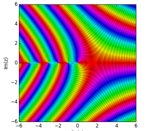
The function is also beautiful when plotted in the complex plane. Here’s a graph where the color corresponds to the complex value of the Gamma function.
At this point, one can feel that we are already lost in abstraction. Perhaps we had initially thought of the factorial as the quantity that tells you about the possible number of permutations of N distinct symbols. But what does it mean to say that there are about -3.676 ways of permuting √2 items, or (.5 – .15 i) ways of permuting an imaginary number of items?
To further frustrate our intuitions, the value of the Gamma function turns out to be undefined at every negative integer. (Some sense can be made of this by realizing that (-1)! is just 0!/0 = 1/0, which is undefined).
Often in times like these, it suits us to switch our intuitive understanding of the factorial to something that does generalize more nicely. Looking at the factorial in the context of probability theory can be helpful.
In statistical mechanics, it is common to describe distributions over events that individually have virtually zero probability of happening, but of which there are virtually infinite opportunities for them to happen, by a Poisson distribution.
An example of this might be a very unlikely radioactive decay. Suppose that the probability p of a single atom decaying is virtually zero, but the number N of atoms in the system you’re studying is virtually infinite ∞, and yet these balance in such a way that the product p∙N = λ is a finite and manageable number.
The Poisson distribution naturally arises as the answer to the question: What is the probability that N atoms decay in a period of time? The form of the distribution is:
P(n) = λn e-λ / n!
We can now use this to imagine a generalization for a process that doesn’t have to be discrete.
Say we are studying the amount of energy emitted in a system where individual emissions have virtually 0 probability but there are a virtually infinite amount of ways for the energy to be emitted. If the energy can take on any real value, then our distribution requires us to talk about the value of n! for arbitrary real n.
Anyway, let’s put aside the attempt to intuitively ground the Gamma function and talk about an application of this to calculus.
Calculus allows us to ask about the derivative of a function, the integral, the second derivative, the 15th derivative, and etc. Lovers of abstraction naturally began to ask questions like: “What’s the ½th derivative of a function? Are there imaginary derivatives?”
This opened the field known as fractional calculus.
Here’s a brief example of how we might do this.
The first derivative D of xn is n xn – 1 The second derivative D2 of xn is n∙(n – 1) ∙ xn – 2 The kth derivative Dk of xn is n! / (n – k)! ∙ xn – k
But we know how to generalize this to any non-integer value, because we know how to generalize the factorial function!
So, for instance, the ½th derivative of x turns out to be:
D½[x] = 1! / ½! ∙ x½ = 2/√π ∙ √x
Now, what we’ve presented is an identity that only applies to functions that look like xn. The general definition for a fractional derivative (or integral) is more complicated, but also uses the Gamma function.
What could it mean to talk about the fractional-derivative of a function? Intuitively, derivatives line up with slopes of curves, second derivatives are slopes of slopes, et cetera. What is a half-derivative of a curve?
I have no way to make intuitive sense of this, although fractional derivatives do tend to line up with our intuitive expectations for what an interpolation between functions should look like.
I’d be interested to know if there are types of functions whose fractional derivatives don’t have this property of smooth transitioning between the ordinary derivatives. Also, I could imagine a generalization of the Taylor approximation, where instead of aligning the integer derivatives of a function, we align all rational derivatives of the function, or all real-valued derivatives from 0 to 1.
The natural next step in this abstraction is to talk about functional calculus, where we can talk about not only arbitrary powers of derivatives, but arbitrary functions of derivatives. In this way we could talk about the logarithm or the sine of a derivative or an integral. But we’ll end the journey into abstraction here, as this ventures into territories that are foreign to me.
Something that seems difficult to me about timeless decision theory is how to reason in a world where most people are not TDTists. In such a world, it seems like the subjunctive dependence between you and others gets weaker and weaker the more TDT influences your decision process.
Suppose you are deciding whether or not to vote. You think through all of the standard arguments you know of: your single vote is virtually guaranteed to not swing the election, so the causal effect of your vote is essentially nothing; the cost to you of voting is tiny, or maybe even positive if you go with a friend and show off your “I Voted” sticker all day; if you vote, you might be able to persuade others to vote as well; etc. At the end of your pondering, you decide that it’s overall not worth it to vote.
Now a TDTist pops up behind your shoulder and says to you: “Look, think about all the other people out there reasoning similarly to you. If you end up not voting as a result of this reasoning, then it’s pretty likely that they’ll all not vote as well. On the other hand, if you do end up voting, then they probably will vote too! So instead of treating your decision as if it only makes the world 1 vote different, you should treat it is if it influences all the votes of those sufficiently similar to you.”
Maybe you instantly find this convincing, and decide to go to the voting booth right away. But the problem is that in taking into account this extra argument, you have radically reduced the set of people whose overall reasoning process is similar to you!
This set was initially everybody that had thought through all the similar arguments and felt similarly to you about them, and most of these people ended up not voting. But as soon as the TDTist popped up and presented their argument, the set of people that were subjunctively dependent upon you shrunk to just those in the initial set that had also heard this argument.
In a world in which only a single person ever had thought about subjunctive dependence, and this person was not going to vote before thinking about it, the evidential effect of not voting is basically zero. Given this, the argument would have no sway on them.
This seems like it would weaken the TDTist’s case that TDTists do better in real world problems. At the same time, it seems actually right. In a case where very few people follow the same reasoning processes as you, your decisions tell you very little about the decisions of others, for the same reason that a highly neuro-atypical person should be hesitant to generalize information about their brain to other people.
Another conclusion of this is that timeless decision theory is most powerful in a community where there is homogeneity of thought and information. Propagation of the idea of timeless decision theory would amplify the coordination-inducing power of the procedure.
I’m not sure if this implies that a TDTist is motivated to spread the idea and homogenize their society, as doing so increases subjunctive dependence and thus enhances their influence. I’d guess that they would only reason this way if they thought themselves to be above average in decision-making, or to have information that others don’t, so that the expected utility of them having increased decision-making ability would outweigh the costs of homogeneity.