Describing the world

February 16, 2020February 16, 2020 ~ ~ 1 Comment

Wittgenstein starts his Tractatus Philosophicus with the following two sentences.

1. The world is everything that is the case.

1.1 The world is the totality of facts, not of things.

Let’s take him up on this suggestion and see how far we get. In the process, we’ll discover some deep connections to theorems in mathematical logic, as well as some fascinating limitations on the expressive powers of propositional and first order logic.

We start out with a set of atomic propositions. For a very simple world, we might only need a finite number of these: “Particle 1 out of 3 has property 1 out of 50”, “Particle 2 of 3 has property 17 out of 50”, and so on. More realistically, the set of atomic propositions will be infinite (countable if the universe doesn’t have any continuous properties, and uncountable otherwise).

For simplicity, we’ll imagine labeling our set of atomic propositions P₁, P₂, P₃, and so on (even though this entails that there are at most countably many, nothing important will rest on this assumption.) We combine these atomic propositions with the operators of propositional logic {(, ), ¬, ∧, ∨, →}. This allows us to build up more complicated propositions, like ((P₇∧P₂)→(¬P₁₃)). This will be the language that we use to describe the world.

Now, the way that the world is is just a consistent assignment of truth values to the set of all grammatical sentences in our language. For example, one simple assignment of truth values is the one that assigns “True” to all atomic propositions. Once we’ve assigned truth values to all the atomic propositions, we get the truth values for the rest of the set of grammatical sentences for free, by the constraint that our truth assignment be consistent. (For instance, if P₁ and P₂ are both true, then (P₁∧P₂) must also be true.)

Alright, so the set of ways the world could be corresponds to the set of truth assignments over our atomic propositions. The final ingredient is the notion that we can encode our present knowledge of the world as a set of sentences. Maybe we know by observation that P₅ is true, and either P₂ or P₃ is true but not both. Then to represent this state of knowledge, we can write the following set of sentences:

{P₅, (P₂∨P₃), ¬(P₂∧P₃)}

Any set of sentences picks out a set of ways the world could be, such that each of these possible worlds is compatible with that knowledge. If you know nothing at all, then the set of sentences representing your knowledge will be the empty set {}, and the set of possible worlds compatible with your knowledge will be the set of all possible worlds (all possible truth assignments). On the other extreme, you might know the truth values of every atomic proposition, in which case your state of knowledge uniquely picks out one possible world.

In general, as you add more sentences to your knowledge-set, you cut out more and more possible worlds. But this is not always true! Ask yourself what the set of possible worlds corresponding to the set {(P₁∨¬P₁), (P₂∨¬P₂), (P₃∨¬P₃)} is. Since each of these sentences is a tautology, no possible worlds are eliminated! So our set of possible worlds is still the set of all worlds.

Now we get to an interesting question: clearly for any knowledge-set of sentences, you can express a set of possible worlds consistent with that knowledge set. But is it the case that for any set of possible worlds, you can find a knowledge-set that uniquely picks it out? If I hand you a set of truth assignment functions and ask you to tell me a set of propositions which are consistent with that set of worlds and ONLY that set, is that always possible? Essentially, what we’re asking is if all sets of possible worlds are describable.

We’ve arrived at the main point of this essay. Take a minute to ponder this and think about whether it’s possible, and why/why not! For clarification, each sentence can only be finitely long. But! You’re allowed to include an infinity of sentences.

(…)

(Spoiler-hiding space…)

(…)

If there were only a finite number of atomic propositions, then you could pick out any set of possible worlds with just a single sentence in conjunctive normal form. But when we start talking about an infinity of atomic propositions, it turns out that it is not always possible! There are sets of possible worlds that are literally not describable, even though our language includes the capacity to describe each of those words and we’re allowed to include an infinite set of sentences.

There’s a super simple proof of this. Let’s give a name to the cardinality of the set of sentences: call it K. (We’ve been tacitly acting as if the cardinality is countable this whole time, but that doesn’t actually matter.) What’s the cardinality of the set of all truth assignments?

Well, each truth assignment is a function from all sentences to {True, False}. And there are 2^K such assignments. 2^K is strictly larger than K, so there are more possible worlds than there are sentences. Now, the cardinality of the set of sets of sentences is also 2^K. But the set of SETS of truth of assignments is 2^{2^K}!

What this means is that we can’t map sets of sentences onto sets of truth assignments without leaving some things out! This proof carries over to predicate logic as well. The language for both propositional and predicate logic is unable to express all sets of possible worlds corresponding to that language!

I love this result. It’s the first hint in mathematical logic that syntax and semantics can come apart.

That result is the climax of this post. What I want to do with the rest of this post is to actually give an explicit example of a set of truth assignments that are “indescribable” by any set of sentences, and to prove it. Warning: If you want to read on, things will get a bit more technical from here.

Alright, so we’ll use a shortcut to denote truth assignments. A truth assignment will be written as a string of “T”s and “F”s, where the nth character corresponds to how the truth assignment evaluates P_n. So the all-true truth assignment will just be written “TTTTTT…” and the all-false truth assignment will be written “FFFFF…”. The truth assignment corresponding to P₁ being false and everything else true will be written “FTTTTT…”. And so on.

Now, here’s our un-describable set of truth assignments. {“FFFFFF…”, “TFFFFF…”, “TTFFFF…”, “TTTFFF…”, …}. Formally, define V_n to be the truth assignment that assigns “True” to every atomic proposition up to and including P_n, and “False” to all others. Now our set of truth assignments is just {V_n | n ∈ ℕ}.

Let’s prove that no set of sentences uniquely picks out this set of truth assignments. We prove by contradiction. Suppose that we could find a set of sentences that uniquely pick out these truth assignments and none other. Let’s call this set A. Construct a new set of sentences A’ by appending all atomic propositions A: A’ = A ∪ {P₁, P₂, P₃, …}.

Is there any truth assignment that is consistent with all of A’? Well, we can answer this by using the Compactness Theorem: A’ has a truth assignment if and only if every finite subset of A’ has a truth assignment. But every finite subset of A’ involves sentences from A (which are consistent with Vn for each n by assumption), and a finite number of atomic propositions. Since each finite subset of A’ is only asserting the truth of a finite number of atomic sentences, we can always find a truth assignment V_k in our set that is consistent with it, by choosing one that switches to “False” long after the last atomic proposition that is asserted by our finite subset.

This means that each finite subset of A’ is consistent with at least one of our truth assignments, which means that A’ is consistent with at least one of our truth assignments. But A’ involves the assertion that all atomic propositions are true! The only truth assignment that is consistent with this assertion is the all-true assignment! And is that truth assignment in our set? No! And there we have it, we’ve reached our contradiction!

We cannot actually describe a set of possible worlds in which either all atomic propositions are false, or only the first is true, or only the first two are true, or only the first three are true, and so on forever. But this might prompt the question: didn’t you just describe it? How did you do that, if it’s impossible? Well, technically I didn’t describe it. I just described the first four possibilities and then said “and so on forever”, assuming that you knew what I meant. To have actually fully pinned down this set of possible worlds, I would have had to continue with this sentence forever. And importantly, since this sentence is a disjunction, I could not split this infinite sentence into an infinite set of finite sentences. This fundamental asymmetry between ∨ and ∧ is playing a big role here: while an infinite conjunction can be constructed by simply putting each clause in the conjunction as a separate sentence, an infinite disjunction cannot be. This places a fundamental limit on the ability of a language with only finite sentences to describe the world.

The full solution to the dog puzzle

February 14, 2020 ~ ~ Leave a comment

A couple of days ago I posted A logic puzzle about dogs. Read that post first and try solving it before reading on!

Below is the full explanation of the puzzle. Heavy spoilers, obviously.

The dog society is structured identically to the Robinson axioms for natural number arithmetic. Dogs are numbers, Spot is 0, the alpha of n is n + 1, the referee for n and m is n + m, the counselor for n and m is n × m, and the strength relation is the < relation. This means that “the marriage counselor for Spot’s alpha and the referee of a fight between Spot’s alpha and Spot’s alpha” is translated to 1 × (1 + 1) = 2, which is Spot’s alpha’s alpha. In Robinson arithmetic, you can also prove that ∀n (n < n + 1).

As for the question of if it’s possible for a dog to be stronger than Spot, Spot’s alpha, Spot’s alpha’s alpha, and so on: The primary difference between Robinson arithmetic and Peano arithmetic (the usual axiomatization of natural numbers) is that the Robinson axioms have no induction axiom (which would be something like “If Spot has a property, and if the alpha of any dog with the property also has the property, then all dogs have the property”). The induction axiom serves to rule out many models of the axioms that are not actually the natural numbers.

If the induction axiom is stated using second-order logic, then the axiom system uniquely pins down (ℕ,+,×,>) and there are no dogs besides those in Spot’s hierarchy. But the induction axiom cannot be stated as a single axiom in first order logic, since it involves quantifying over all properties. For first-order Peano arithmetic, we instead have an infinite axiom schema, one for each property that is definable within the first-order language. This turns out to be strictly weaker than the single second-order axiom, as there are some properties of numbers that cannot be described in a first-order language (like being larger than a finite number of numbers).

What this amounts to is that first-order Peano arithmetic with its infinite axiom schema is too weak to pin down the natural numbers as a unique model. There are what’s called nonstandard models of first order PA, which contains the ordinary numbers but also an infinity of weird extra numbers.(In fact, there exist models of first-order PA with every infinite cardinality!) Some of these numbers have the property that they are bigger than all the regular natural numbers.And since Robinson arithmetic is strictly weaker than first-order PA (lacking an induction axiom as it does), this means that Robinson arithmetic is also not strong enough to rule out numbers greater than all elements of ℕ. Which means that we cannot prove that there are no dogs stronger than every dog in Spot’s hierarchy!

I made this puzzle to illustrate three things: First, how the same axioms, and even the same models of the same axioms, can have wildly different interpretations, and that a shift in how you think about these axioms can make seemingly impossible tasks trivial. Second, how axiom systems for structures like ℕ can (and inevitably do) fail to capture important and intuitively obvious features of the structure. And third, how logic is so interesting! Just trying to create a simple rule system to describe one of the most natural and ordinary mathematical structures that we ALL use ALL THE TIME for reasoning about the world, turns out to be so nontrivial, and in fact impossible to do perfectly!

Three paradoxes of self-reference

February 11, 2020 ~ ~ 2 Comments

I’ve spent a lot of time in the past describing the paradoxes that arise when we try to involve infinities into our reasoning. Another way to get paradoxes aplenty is by invoking self-reference. Below are three of the best paradoxes of self-reference for you to sort out.

In each case, I want you to avoid the temptation to just say “Ah, it’s just self-reference that’s causing the problem” and feel that the paradox is thus resolved. After all, there are plenty of benign cases of self-reference. Self-modifying code, flip-flops in computing hardware, breaking the fourth wall in movies, and feeding a function as input to itself are all examples. Self-referential definitions in mathematics are also often unobjectionable: as an example, we can define the min function by saying y = min(X) iff y is in X and for all elements x of X, y ≤ x (the definition quantifies over a group of objects that includes the thing being defined). So if we accept that self-reference is not necessarily paradoxical (just as infinity is sometimes entirely benign), then we must do more to resolve the below paradoxes than just say “self-reference.”

1. Berry’s Paradox

Consider the set of integers definable in an English sentence of under eighty letters. This set is finite, because there are only a finite number of possible strings of English characters of under eighty letters. So since this set is finite and there are an infinity of integers, there must be a smallest integer that’s not in the set.

But hold on: “The smallest positive integer not definable in under eighty letters” appears to now define this integer, and it does so with only 67 letters! So now it appears that there is no smallest positive integer not definable in under eighty letters. And that means that our set cannot be finite! But of course, the cardinality of the set of strings cannot be less than the cardinality of the set of numbers those strings describe. So what’s going on here?

2. Curry’s paradox

“If this sentence is true, then time is infinite.”

Curry’s paradox tells us that just from the existence of this sentence (assuming nothing about its truth value), we can prove that time is infinite.

Proof 1

Let’s call this sentence P. We can then rewrite P as “If P is true, then time is infinite.” Now, let’s suppose that the sentence P is true. That means the following:

Under the supposition that P is true, it’s true that “If P is true, then time is infinite.”

And under the supposition that P is true, P is true.

So under the supposition that P is true, time is infinite (by modus ponens within the supposition).

But this conclusion we’ve just reached is just the same thing as P itself! So we’ve proven that P is true.

And therefore, since P is true and “If P is true, then time is infinite” is true, time must be infinite!

If you’re suspicious of this proof, here’s another:

Proof 2

If P is false, then it’s false that “If P is true then time is infinite.” But the only way that sentence can be false is if the antecedent is true and the consequent false, i.e. P is true and time is finite. So from P’s falsity, we’ve concluded P’s truth. Contradiction, so P must be true.

Now, if P is true, then it’s true that “If P is true, then time is infinite”. But then by modus ponens, time must be infinite.

Nothing in our argument relied on time being infinite or finite, so we could just as easily substitute “every number is prime” for “time is infinite”, or anything we wanted. And so it appears that we’ve found a way to prove the truth any sentence! Importantly, our conclusion doesn’t rest on the assumption of the truth of the sentence we started with! All it requires is the *existence of the sentence*. Is this a proof of the inconsistency of propositional logic? And if not, then where exactly have we gone wrong?

3. Curry’s paradox, Variant

Consider the following two sentences:

1) At least one of these two sentences is false.
2) Not all numbers are prime.

Suppose that (1) is false. Well then at least one of the two sentences is false, which makes (1) true! This is a contradiction, so (1) must be true.

Since (1) is true, at least one of the two sentences must be false. But since we already know that (1) is true, (2) must be false. Which means that all numbers are prime!

Just like last time, the structure of the argument is identical no matter what we put in place of premise 2, so we’ve found a way to disprove any statement! And again, we didn’t need to start out by assuming anything about the truth values of sentences (1) and (2), besides that they have truth values.

Perhaps the right thing to say, then, is that we cannot always be sure that self-referential statements actually have truth values. But then we have to answer the question of how we are to distinguish between self-referential statements that are truth-apt and those that are not! And that seems very non-trivial. Consider the following slight modification:

1) Both of these two sentences are true.
2) Not all numbers are prime.

Now we can just say that both (1) and (2) are true, and there’s no problem! And this seems quite reasonable; (1) is certainly a meaningful sentence, and it seems clear what the conditions for its truth would be. So what’s the difference in the case of our original example?

A logic puzzle about dogs

February 10, 2020February 11, 2020 ~ ~ 1 Comment

Spot is a dog. Every dog has one alpha (also a dog), and no two dogs have the same alpha. But Spot, alone amongst dogs, isn’t anybody’s alpha. 😦

For any two dogs, there is an assigned referee in case they get into a fight and an assigned marriage counselor in case they get married. The dogs have set up the following rules for deciding who will be the referees and counselors for who:

If Spot fights with any dog, the other dog gets to be the referee. The referee of a fight between dog 1’s alpha and dog 2 has to be the alpha of the referee of a fight between dogs 1 and 2.

Spot has to be his own marriage counselor, no matter who he marries. The marriage counselor for dog 1’s alpha and dog 2 has to referee any fight between dog 2 and the marriage counselor for dog 1 and dog 2.

Finally, dog 1 is stronger then dog 2 if and only if dog 1 is the referee for dog 2 and some other dog. Strength is transitive, and no dog is stronger than itself.

Question 1: Who’s the marriage counselor for Spot’s alpha and the referee of a fight between Spot’s alpha and Spot’s alpha?

Question 2: How many dogs are there?

Question 3: Is the referee for dog 1’s alpha and dog 2 always the same as the referee for dog 2’s alpha and dog 1? What if we asked the same question about marriage counselors?

Question 4: Is any dog stronger than their own alpha?

Bonus Question: Is it possible for there to be a dog that’s stronger than Spot, Spot’s alpha, Spot’s alpha’s alpha, and so on?

A challenge: Try to figure out a trick that allows you to figure out the above questions in your head. I promise, it’s possible!

A suspicious proof of God’s existence

February 9, 2020 ~ ~ 4 Comments

Consider the following argument:

If I will have eternal life if I believe in God, then God must exist.
I do not believe in God.
Therefore, God exists.

Intuitively, it seems possible for (1) and (2) to be true and yet (3) to be false.

But now let’s formalize the argument.

B = “I believe in God”
E = “I will get eternal life”
G = “God exists”

(B → E) → G
~B
Assume ~G
~(B → E), modus tollens (1,3)
B & ~E, (4)
B, (5)
B & -B, (6,2)
G, proof by contradiction (2 through 7)

This argument is definitely logically valid, so were our initial intuitions mistaken? And if not, then what’s going on here?

Fractal Trees

February 8, 2020April 16, 2026 ~ ~ 2 Comments

Consider the following simple algorithm:

We start with a single painted particle moving upwards at a decreasing velocity, with a trajectory that is slowly rotating at a constant velocity. At each step, there is some small probability for the particle to “split” into two particles, one of which begins rotating in the opposite direction. And if a particle’s trajectory is ever about to start turning downwards, it instead reverses its angular velocity and begins turning upwards.

Those are all the rules. So what sort of shapes does this incredibly simple algorithm generate? Take a look!

$fracTree_1$ $fracTree_2$ $fracTree_4$

And for one last animation, let’s allow the particles to have a downwards-facing trajectory to get a different type of tree:

$fracTree_5$

It might be unbelievable that such a simple algorithm could generate such complex and organic shapes, but you can try it for yourself: the images above are produced by only 25 lines of code! And of course, it makes one very curious about whether there is a real connection between this algorithm and the way that plants actually grow.

Diversification is magic

December 11, 2019 ~ ~ 1 Comment

“The only free lunch in finance is diversification”

Harry Markowitz

Suppose you have two assets that you can invest in, and $1000 dollars total to split between them. By the end of year 1, Asset A doubles in price and Asset B halves in price. And by the end of year 2, A halves and B doubles (so that they each return to their starting point).

Diversify

If you had initially invested all $1000 in Asset A, then after year 1 you would have $2000 total. But after year 2, that $2000 is cut in half and you end up back at $1000. If you had invested the $1000 in Asset B, then you would go down to $500 after year 1 and then back up to $1000 after year 2. Either way, you don’t get any profit.

Now, the question is: can you find some way to distribute the $1000 dollars across Assets A and B such that by the end of year 2 you have made a profit? For fairness sake, you cannot change your distribution at the end of year 1 (as that would allow you to take advantage of the advance knowledge of how the prices will change). Whatever weights you choose initially for Assets A and B, at the end of year 1 you must move around your money so that you ensure it’s still distributed with the exact same weights as before.

So what do you think? Does it seem impossible to make a profit without changing your distribution of money between years 1 and 2? Amazingly, the answer is that it’s not impossible; you can make a profit!

Consider a 50/50 mix of Assets A and B. So $500 initially goes into Asset A and $500 to Asset B. At the end of year 1, A has doubled in price (netting you $500) and B has halved (losing you $250). So at the end of year 1 you have gained 25%.

To keep the weights the same at the start of year 2 as they were at the start of year 1, you redistribute your new total of $1250 across A and B according to the same 50/50 mix ($625 in each). What happens now? Now Asset A halves (losing you $312.50) and Asset B doubles (gaining you $625). And by the end of year 2, you end up with $312.50 in A and $1250 in B, for a total of $1562.50! You’ve gained $562.50 by investing in two assets whose prices ultimately are the same as where they started!

Diversify 2

This is the magic of diversification. By investing in multiple independent assets instead of just one, you can up your rate of return and decrease your risk, sometimes dramatically.

Another example: In front of you are two fair coins, A and B. You have in your hand $100 that you can distribute between the two coins any way you like, so long as all $100 is on the table. Now, each of the coins will be tossed. If a coin lands heads, the amount of money beside it will be doubled and returned to you. But if the coin lands tails, then all the money beside it will be destroyed.

In front of you are two coins, A and B. You have $100 dollars to distribute between these two coins. You get to choose how to distribute the $100, but at the end every dollar bill must be beside one coin or the other.

Coin A has a 60% chance of landing H. If it lands H, the amount of money placed beside it will be multiplied by 2.1 and returned to you. But if it lands T, then the money placed beside it will be lost.

Coin B has only a 40% chance of landing H. But the H outcome also has a higher reward! If the coin lands H, then the amount of money beside it will be multiplied by 2.5 and returned to you. And just like Coin A, if it lands T then the money beside it will be destroyed.

Coin A: .6 chance of getting 2.1x return
Coin B: .4 chance of getting 2.5x return

The coins are totally independent. How should you distribute your money in order to maximize your return, given a specific level of risk?

(Think about it for a moment before reading on.)

If you looked at the numbers for a few moments, you might have noticed that Coin A has a higher expected return than Coin B (126% vs 100%) and is also the safer of the two. So perhaps your initial guess was that putting everything into Coin A would minimize risk and maximize return. Well, that’s incorrect! Let’s do the math.

We’ll start by giving the relevant quantities some names.

X = amount of money that is put by Coin A
Y = amount of money that is put by Coin B
(All your money is put down, so Y = 100 – X)

We can easily compute the expected amount of money you end up with, as a function of X:

Expected return (X)
= (0.6)(0.4)(2.1X + 2.5Y) + (0.6)(0.6)(2.1X) + (0.4)(0.4)(2.5Y) + (0.4)(0.6)(0)
= 100 + .26 X

Alright, so clearly your expected return is maximized by making X as large as possible (by putting all of your money by Coin A). This makes sense, since Coin A’s expected return is higher than Coin B’s. But we’re not just interested in return, we’re also interested in risk. Could we possibly find a better combination of risk and reward by mixing our investments? It might initially seem like the answer is no; after all Coin A is the safer of the two. How could we possibly decrease risk by mixing in a riskier asset to our investments?

The key insight is that even though Coin A is the safer of the two, the risk of Coin B is uncorrelated with the risk of Coin A. If you invest everything in Coin A, then you have a 40% chance of losing it all. But if you split your investments between Coin A and Coin B, then you only lose everything if both coins come up heads (which happens with probability .6*.4 = 24%, much lower than 40%!)

Let’s go through the numbers. We’ll measure risk by the standard deviation of the possible outcomes.

Risk(X)²
= (0.6)(0.4)(2.1X + 2.5Y – 100 – .26X)² + (0.6)(0.6)(2.1X – 100 – .26X)² + (0.4)(0.4)(2.5Y – 100 – .26X)² + (0.4)(0.6)(0 – 100 – .26X)²

This function is just a parabola (to be precise, Risk² is a parabola, which means that Risk(x) is a hyperbola). Here’s a plot of Risk(X) vs X (amount placed beside A):

Diversify Risk v X

Looking at this plot, you can see that risk is actually minimized at a roughly even mix of A and B, with slightly more in B. You can also see this minimum risk on a plot of return vs risk:

Notice that somebody that puts most of their money on coin B (these mixes are in the bottom half of the curve) is making a strategic choice is strictly dominated. That is, they could choose a different mix that has a higher rate of return for the same risk!

Little did you know, but you’ve actually just gotten an introduction to modern portfolio theory! Instead of putting money beside coins, portfolio managers consider investing in assets with various risks and rates of return. The curve of reward vs risk is famous in finance as the Markowitz Bullet. The upper half of the curve is the set of portfolios that are not strictly dominated. This section of the curve is known as the efficient frontier, the basic idea being that no rational investor would put themselves on the lower half.

Let’s reframe the problem in terms that would be familiar to somebody in finance.

We have two assets, A and B. We’ll model our knowledge of the rate of return of each asset as a normal distribution with some known mean and standard deviation. The mean of the distribution represents the expected rate of return on a purchase of the asset, and the standard deviation represents the risk of purchasing the asset. Asset A has an expected rate of return of 1.2, which means that for every dollar you put in you expect (on average) to get back $0.20 a year from now. Asset B’s expected rate of return is 1.3, so it has a higher average payout. But Asset B is riskier; the standard deviation for A is 0.5, while B’s standard deviation is 0.8. There’s also a risk-free asset that you can invest in, which we’ll call Asset F. This asset has an expected rate of return of 1.1.

Asset F: R = 1.1, σ = 0
Asset A: R = 1.2, σ = 0.5
Asset B: R = 1.3, σ = 0.8

Suppose that you have $1000 that you want to invest in some combination of these three assets in such a way as to maximize your expected rate of return and minimize your risk. Since rate of return and risk will in general be positively correlated, you have to decide the highest risk that you’re comfortable with. Let’s say that you decide that the highest risk you’ll accept is 0.6. Now, how much of each asset should you purchase?

First of all, let’s disregard the risk-free asset and just consider combinations of A and B. A portfolio of A and B is represented by the weighted sum of A and B. w_A is the percentage of your investment in the portfolio that goes to just A, and w_B is the percentage that goes towards B. Since we’re just considering a combination of A and B for now, w_A + w_B = 1. The mean and standard deviation of the new distribution for this portfolio will in general depend on the correlation between A and B, which we’ll call ρ. Perfectly correlated assets have ρ = 1, uncorrelated assets have ρ = 0, and perfectly anti-correlated assets have ρ = -1. Correlation between assets is bad for investors, because it destroys the benefit of diversification. If two assets are perfectly correlated, then you don’t get any lower risk by combining them. On the other hand, if they are perfectly anti-correlated, you can entirely cancel the risk from one with the risk from the other, and get fantastically low risks for great rates of return.

R_P = w_AR_A + w_BR_B
σ_P² = w_A²σ_A² + w_B²σ_B² + 2ρw_Aw_Bσ_Aσ_B

Let’s suppose that the correlation between A and B is ρ = .2. Since both R_P and σ_P are functions of w_A and w_B, we can visualize the set of all possible portfolios as a curve on a plot of return-vs-risk:

The Markowitz Bullet again! Each point on the curve represents the rate of return and risk of a particular portfolio obtained by mixing A and B. Just like before, some portfolios dominate others and thus should never be used, regardless of your desired level of risk. In particular, for any portfolio that weights asset A (the less risky one) too highly, there are other portfolios that give a higher rate of return with the exact same risk.

In other words, you should pretty much never purchase only a low-risk low-return item. If your portfolio consists entirely of Asset A, then by mixing in a little bit of the higher-risk item, you can actually end up massively decreasing your risk and upping your rate of return. Of course, this drop in risk is only because the two assets are not perfectly correlated. And it would be even more extreme if we had negatively correlated assets; indeed with perfect negative correlation (as we saw in the puzzle I started this post with), your risk can drop to zero!

Now, we can get our desired portfolio with a risk of 0.6 by just looking at the point on this curve that has σ_P = 0.6 and calculating which values of w_A and w_B give us this value. But notice that we haven’t yet used our riskless asset! Can we do better by adding in a little of Asset F to the mix? It turns out that yes, we can. In fact, every portfolio is weakly dominated by some mix of that portfolio and a riskless asset!

We can easily calculate what we get by combining a riskless asset with some other asset X (which can in general be a portfolio consisting of multiple assets):

R_P = w_XR_X + w_FR_F
σ_P² = w_X²σ_X² + w_F²σ_F² + 2ρw_Xw_Fσ_Xσ_F = w_X²σ_X²

So σ_P = w_Xσ_X, from which we get that R_P = (σ_P/σ_X)R_X + (1 – σ_P/σ_X)R_F = R_F + σ_P (R_X – R_F)/σ_X

What we find is that R_P(σ_P) is just a line whose slope depends on the rate of return and risk of asset X. So essentially, for any risky asset or portfolio you choose, you can easily visualize all the possible ways it can be combined with a risk-free asset by stretching a line from (0, R_F) – the risk and return of the risk-free asset – to (s_X, R_X) – the risk and return of the risky asset. We can even stretch the line beyond this second point by borrowing some of the risk-free asset in order to buy more of the risky asset, which corresponds to a negative weighting w_F.

So, we have a quadratic curve representing the possible portfolios obtained from two risky assets, and a line representing the possible portfolios obtained from a risky asset and a risk-free asset. What we can do now is consider the line that starts at (0, R_F) and just barely brushes against the quadratic curve – the tangent line to the curve that passes through (0, R_F). This point where the curves meet is known as the tangency portfolio.

Every point on this line is a possible combination of Assets A, B, and F. Why? Well, because the points on the line can be thought of as portfolios consisting of Asset F and the tangency portfolio. And here’s the crucial point: this line is above the curve everywhere except at that single point! What this means is that the combination of A, B, and F dominates combinations of just A and B. For virtually any level of desired risk, you do better by choosing a portfolio on the line than by choosing the portfolio on the quadratic curve! (The only exception to this is the point at which the two curves meet, and in that case you do equally well.)

And that is how you optimize your rate of return for a desired level of risk! First generate the hyperbola for portfolios made from your risky assets, then find the tangent to that curve that passes through the point representing the risk-free asset, and then use that line to calculate the optimal portfolio at your chosen level of risk!

Solving the Linear Cournot Model

December 2, 2019December 2, 2019 ~ ~ 3 Comments

The Cournot model is a simple economic model used to describe what happens when multiple companies compete with one another to produce some homogenous product. I’ve been playing with it a bit and ended up solving the general linear case. I assume that this solution is already known by somebody, but couldn’t find it anywhere. So I will post it here! It gives some interesting insight into the way that less-than-perfectly-competitive markets operate. First let’s talk about the general structure of the Cournot model.

Suppose we have n firms. Each produces some quantity of the product, which we’ll label as $q_1, q_2, ..., q_n$ . The total amount of product on the market will be given the label $Q = q_1 + q_2 + ... + q_n$ . Since the firms are all selling identical products, it makes sense to assume that the consumer demand function $P(q_1, q_2, ..., q_n)$ will just be a function of the total quantity of the product that is on the market: $P(q_1, q_2, ..., q_n) = P(q_1 + q_2 + ... + q_n) = P(Q)$ . (This means that we’re also disregarding effects like customer loyalty to a particular company or geographic closeness to one company location over another. Essentially, the only factor in a consumer’s choice of which company to go to is the price at which that company is selling the product.)

For each firm, there is some cost to producing the good. We capture this by giving each firm a cost function $C_1(q_1), C_2(q_2), ..., C_n(q_n)$ . Now we can figure out the profit of each firm for a given set of output values $q_1, q_2, ..., q_n$ . We’ll label the profit of the kth firm as $\Pi_k$ . This profit is just the amount of money they get by selling the product minus the cost of producing the product: $\Pi_k = q_k P(Q) - C_k(q_k)$ .

If we now assume that all firms are maximizing profit, we can find the outputs of each firm by taking the derivative of the profit and setting it to zero. $\frac{d\Pi_k}{dq_k} = P(Q) + q_k \frac{dP}{dQ} - \frac{dC_k}{dq_k} = 0$ . This is a set of n equations with n unknown, so solving this will fully specify the behavior of all firms!

Of course, without any more assumptions about the functions $P$ and $C_k$ , we can’t go too much further with solving this equation in general. To get some interesting general results, we’ll consider a very simple set of assumptions. Our assumptions will be that both consumer demand and producer costs are linear. This is the linear Cournot model, as opposed to the more general Cournot model.

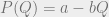
In the linear Cournot model, we write that $P(Q) = a - bQ$ (for some a and b) and $C_k(q_k) = c_k q_k$ . As an example, we might have that P(Q) = $100 – $2 × Q, which would mean that at a price of $40, 30 units of the good will be bought total.

demand curve.png

The constants $c_k$ represent the marginal cost of production for each firm, and the linearity of the cost function means that the cost of producing the next unit is always the same, regardless of how many have been produced before. (This is unrealistic, as generally it’s cheaper per unit to produce large quantities of a good than to produce small quantities.)

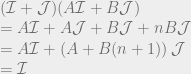
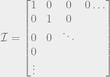
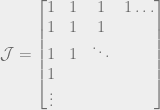
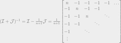
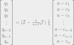
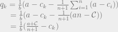
Now we can write out the profit-maximization equations for the linear Cournot model. $\frac{d\Pi_k}{dq_k} = P(Q) + q_k \frac{dP}{dQ} - \frac{dC_k}{dq_k} = a - bQ - b q_k - c_k = 0$ . Rewriting, we get $q_k + Q = \frac{a - c_k}{b}$ . We can’t immediately solve this for $q_k$ , because remember that Q is the sum of all the quantities produced. All n of the quantities we’re trying to solve are in each equation, so to solve the system of equations we have to do some linear algebra!

$2q_1 + q_2 + q_3 + ... + q_n = \frac{a - c_1}{b} \\ q_1 + 2q_2 + q_3 + ... + q_n = \frac{a - c_2}{b} \\ q_1 + q_2 + 2q_3 + ... + q_n = \frac{a - c_2}{b} \\ \ldots \\ q_1 + q_2 + q_3 +... + 2q_n = \frac{a - c_n}{b}$

Translating this to a matrix equation…

$\begin{bmatrix} 2 & 1 & 1 & 1 & 1 & \ldots \\ 1 & 2 & 1 & 1 \\ 1 & 1 & 2 & & \ddots \\ 1 & 1 & & \ddots \\ 1 & & \ddots \\ \vdots \end{bmatrix} \begin{bmatrix} q_1 \\ q_2 \\ q_3 \\ \vdots \\ q_{n-2} \\ q_{n-1} \\ q_n \end{bmatrix} = \frac{1}{b} \begin{bmatrix} a - c_1 \\ a - c_2 \\ a - c_3 \\ \vdots \\ a - c_{n-2} \\ a - c_{n-1} \\ a - c_n \end{bmatrix}$

Now if we could only find the inverse of the first matrix, we’d have our solution!

$\begin{bmatrix} q_1 \\ q_2 \\ q_3 \\ \vdots \\ q_{n-2} \\ q_{n-1} \\ q_n \end{bmatrix} = \begin{bmatrix} 2 & 1 & 1 & 1 & 1 & \ldots \\ 1 & 2 & 1 & 1 \\ 1 & 1 & 2 & & \ddots \\ 1 & 1 & & \ddots \\ 1 & & \ddots \\ \vdots \end{bmatrix} ^{-1} \frac{1}{b} \begin{bmatrix} a - c_1 \\ a - c_2 \\ a - c_3 \\ \vdots \\ a - c_{n-2} \\ a - c_{n-1} \\ a - c_n \end{bmatrix}$

I found the inverse of this matrix by using the symmetry in the matrix to decompose it into two matrices that were each easier to work with:

$\mathcal{I} = \begin{bmatrix} 1 & 0 & 0 & 0 \ldots \\ 0 & 1 & 0 \\ 0 & 0 & \ddots \\ 0 \\ \vdots \end{bmatrix}$

$\mathcal{J} = \begin{bmatrix} 1 & 1 & 1 & 1 \ldots \\ 1 & 1 & 1 \\ 1 & 1 & \ddots \\ 1 \\ \vdots \end{bmatrix}$

$\begin{bmatrix} 2 & 1 & 1 & 1 & 1 & \ldots \\ 1 & 2 & 1 & 1 \\ 1 & 1 & 2 & & \ddots \\ 1 & 1 & & \ddots \\ 1 & & \ddots \\ \vdots \end{bmatrix} = \mathcal{I} + \mathcal{J}$

As a hypothesis, suppose that the inverse matrix has a similar form (one value for the diagonal elements, and another value for all off-diagonal elements). This allows us to write an equation for the inverse matrix:

$(\mathcal{I} + \mathcal{J}) (A \mathcal{I} + B \mathcal{J}) = \mathcal{I}$

To solve this, we’ll use the following easily proven identities.

$\mathcal{I} \cdot \mathcal{I} = \mathcal{I} \\ \mathcal{I} \cdot \mathcal{J} = \mathcal{J} \\ \mathcal{J} \cdot \mathcal{I} = \mathcal{J} \\ \mathcal{J} \cdot \mathcal{J} = n \mathcal{J} \\$

$(\mathcal{I} + \mathcal{J}) (A \mathcal{I} + B \mathcal{J}) \\ = A \mathcal{I} + A \mathcal{J} + B \mathcal{J} + nB \mathcal{J} \\ = A \mathcal{I} + \left( A + B(n+1) \right) \mathcal{J} \\ = \mathcal{I}$

$A = 1 \\ A + B(n+1) = 0$

$A = 1 \\ B = - \frac{1}{n+1}$

$(\mathcal{I} + \mathcal{J})^{-1} = \mathcal{I} - \frac{1}{n+1} \mathcal{J} = \frac{1}{n+1} \begin{bmatrix} n & -1 & -1 & -1 & -1 & \ldots \\ -1 & n & -1 & -1 \\ -1 & -1 & n & & \ddots \\ -1 & -1 & & \ddots \\ -1 & & \ddots \\ \vdots \end{bmatrix}$

Alright awesome! Our hypothesis turned out to be true! (And it would have even if the entries in our matrix hadn’t been 1s and 2s. This is a really cool general method to find inverses of this family of matrices.) Now we just use this inverse matrix to solve for the output from each firm!

$\begin{bmatrix} q_1 \\ q_2 \\ q_3 \\ \vdots \\ q_{n-2} \\ q_{n-1} \\ q_n \end{bmatrix} = (\mathcal{I} - \frac{1}{n+1} \mathcal{J}) \ \frac{1}{b} \begin{bmatrix} a - c_1 \\ a - c_2 \\ a - c_3 \\ \vdots \\ a - c_{n-2} \\ a - c_{n-1} \\ a - c_n \end{bmatrix}$

Define: $\mathcal{C} = \sum_{i=1}^{n}{c_i}$

$q_k = \frac{1}{b} (a - c_k - \frac{1}{n+1} \sum_{i=1}^{n}{(a - c_i)}) \\ ~~~~ = \frac{1}{b} (a - c_k - \frac{1}{n+1} (an - \mathcal{C})) \\ ~~~~ = \frac{1}{b} (\frac{a + \mathcal{C}}{n+1} - c_k)$

$Q^* = \sum_{k=1}^n {q_k} \\ ~~~~~ = \frac{1}{b} \sum_{k=1}^n ( \frac{a + \mathcal{C}}{n+1} - c_k ) \\ ~~~~~ = \frac{1}{b} \left( \frac{n}{n+1} (a + \mathcal{C}) - \mathcal{C} \right) \\ ~~~~~ = \frac{1}{b} \left( \frac{n}{n+1} a - \frac{\mathcal{C}}{n+1} \right) \\ ~~~~~ = \frac {an - \mathcal{C}} {b(n+1)}$

$P^* = a - bQ^* \\ ~~~~~ = a - \frac{an - \mathcal{C}}{n+1} \\ ~~~~~ = \frac{a + \mathcal{C}}{n+1}$

$\Pi_k^* = q_k^* P^* - c_k q_k^* \\ ~~~~~ = \frac{1}{b} (\frac{a+\mathcal{C}}{n+1} - c_k) \frac{a + \mathcal{C}}{n+1} - \frac{c_k}{b} (\frac{a + \mathcal{C}}{n+1} - c_k) \\ ~~~~~ = \frac{1}{b} \left( \left( \frac{a + \mathcal{C}}{n+1} \right)^2 - 2c_k\left( \frac{a + \mathcal{C}}{n+1} \right) + c_k^2 \right) \\ ~~~~~ = \frac{1}{b} \left( \frac{a + \mathcal{C}}{n+1} - c_k \right)^2$

And there we have it, the full solution to the general linear Cournot model! Let’s discuss some implications of these results. First of all, let’s look at the two extreme cases: monopoly and perfect competition.

Monopoly: n = 1
$Q^* = \frac{1}{2b} (a - c) \\ P^* = \frac{1}{2} (a + c) \\ \Pi^* = \frac{1}{b} \left( \frac{a - c}{2} \right)^2$

Perfect Competition: n → ∞
$q_k^* \rightarrow \frac{1}{b} (\bar c - c_k) \\ Q^* \rightarrow \frac{1}{b} (a - \bar c) \\ P^* \rightarrow \bar c \\ \Pi^* \rightarrow \frac{1}{b} (\bar c - c_k)^2$

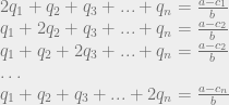
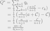
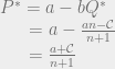
The first observation is that the behavior of the market under monopoly looks very different from the case of perfect competition. For one thing, notice that the price under perfect competition is always going to be lower than the price under monopoly. This is a nice demonstration of the so-called monopoly markup. The quantity $a$ intuitively corresponds to the highest possible price you could get for the product (the most that the highest bidder would pay). And the quantity $c$ , the production cost, is the lowest possible price at which the product would be sold. So the monopoly price is the average of the highest price you could get for the good and the lowest price at which it could be sold.

The flip side of the monopoly markup is that less of the good is produced and sold under a monopoly than under perfect competition. There are trades that could be happening (trades which would be mutually beneficial!) which do not occur. Think about it: the monopoly price is halfway between the cost of production and the highest bidder’s price. This means that there are a bunch of people that would buy the product at above the cost of production but below the monopoly price. And since the price they would buy it for is above the cost of production, this would be a profitable exchange for both sides! But alas, the monopoly doesn’t allow these trades to occur, as it would involve lowering the price for everybody, including those who are willing to pay a higher price, and thus decreasing net profit.

Things change as soon as another firm joins the market. This firm can profitably sell the good at a lower price than the monopoly price and snatch up all of their business. This introduces a downward pressure on the price. Here’s the exact solution for the case of duopoly.

Duopoly: n = 2
$q_1 = \frac{1}{3b} (a - 2c_1 + c_2) \\ q_2 = \frac{1}{3b} (a + c_1 - 2c_2) \\ Q^* = \frac{1}{3b} (2a - c_1 - c_2) \\ P^* = \frac{1}{3} (a + c_1 + c_2) \\ \Pi_1^* = \frac{1}{3b} (a - 2c_1 + c_2)^2 \\ \Pi_2^* = \frac{1}{3b} (a + c_1 - 2c_2)^2 \\$

Interestingly, in the duopoly case the market price still rests at a value above the marginal cost of production for either firm. As more and more firms enter the market, competition pushes the price down further and further until, in the limit of perfect competition, it converges to the cost of production.

The implication of this is that in the limit of perfect competition, firms do not make any profit! This may sound a little unintuitive, but it’s the inevitable consequence of the line of argument above. If a bunch of companies were all making some profit, then their price is somewhere above the cost of production. But this means that one company could slightly lower its price, thus snatching up all the customers and making massively more money than its competitors. So its competitors will all follow suit, pushing down their prices to get back their customers. And in the end, all the firms will have just decreased their prices and their profits, even though every step in the sequence appeared to be the rational and profitable action by each firm! This is just an example of a coordination problem. If the companies could all just agree to hold their price fixed at, say, the monopoly price, then they’d all be better off. But each individual has a strong monetary incentive to lower their price and gather all the customers. So the price will drop and drop until it can drop no more (that is, until it has reached the cost of production, at which point it is no longer profitable for a company to lower their price).

This implies that in some sense, the limit of perfect competition is the best possible outcome for consumers and the worst outcome for producers. Every consumer that values the product above the cost of its production will get it, and they will all get it at the lowest possible price. So the consumer surplus will be enormous. And companies producing the product make no net profit; any attempt to do so immediately loses them their entire customer base. (In which case, what is the motivation for the companies to produce the product in the first place? This is known as the Bertrand paradox.)

We can also get the easier-to-solve special case where all firms have the same cost of production.

Equal Production Costs
$\forall k (c_k = c)$
$q_k^* = \frac{1}{n+1} \frac{a - c}{b} \\ Q^* = \frac{n}{n+1} \frac{a - c}{b} \\ P^* = \frac{a + nc}{n + 1} \\ \Pi^* = \frac{1}{b} \left( \frac{a - c}{n+1} \right)^2$

It’s curious that in the Cournot model, prices don’t immediately drop to production levels as soon you go from a monopoly to a duopoly. After all, the intuitive argument I presented before works for two firms: if both firms are pricing the goods at any value above zero, then each stands to gain by lowering the price a slight bit and getting all the customers. And this continues until the price settles at the cost of production. We didn’t build in any ability of the firms to collude to the model, so what gives? What the Cournot model tells us is certainly more realistic (we don’t expect a duopoly to behave like a perfectly competitive market), but where does this realism come from?

The answer is that in a certain sense we did build in collusion between firms from the start, in the form of agreement on what price to sell at. Notice that our model did not allow different firms to set different prices. In this model, firms compete only on quantity of goods sold, not prices. The price is set automatically by the consumer demand function, and no single individual can unilaterally change their price. This constraint is what gives us the more realistic-in-character results that we see, and also what invalidates the intuitive argument I’ve made here.

One final observation. Consider the following procedure. You line up a representative from each of the n firms, as well as the highest bidder for the product (representing the highest price at which the product could be sold). Each of the firms states their cost of production (the lowest they could profitably bring the price to), and the highest bidder states the amount that he values the product (the highest price at which he would still buy it). Now all of the stated costs are averaged, and the result is set as the market price of the good. Turns out that this procedure gives exactly the market price that the linear Cournot model predicts! This might be meaningful or just a curious coincidence. But it’s quite surprising to me that the slope of the demand curve ( $b$ ) doesn’t show up at all in the ultimate market price, only the value that the highest bidder puts on the product!

Building an analog calculator

November 25, 2019April 16, 2026 ~ ~ 1 Comment

Op-amps are magical little devices that allow us to employ the laws of electromagnetism for our purposes, giving us the power to do ultimately any computation using physics. To explain this, we need to take three steps: first transistors, then differential amplifiers, and then operational amplifiers. The focus of this post will be on purely analog calculations, as that turns out to be the most natural type of computation you get out of op amps.

1. Transistor

Here’s a transistor:

It has three ports, named (as labelled) the base, the collector and the emitter. Intuitively, you can think about the base as being like a dial that sensitively controls the flow of large quantities of current from the collector to the emitter. This is done with only very small trickles of current flowing into the base.

More precisely, a transistor obeys the following rules:

The transistor is ON if the voltage at the collector is higher than the voltage at the emitter. It is OFF otherwise.
When the transistor is in the ON state, which is all we’ll be interested in, the following regularities are observed:
1. Current flows along only two paths: base-to-emitter and collector-to-emitter. A transistor does not allow current to flow from the emitter to either the collector or the base.
2. The current into the collector is proportional to the current into the base, with a constant of proportionality labelled β whose value is determined by the make of the transistor. β is typically quite large, so that the current into the collector is much larger than the current into the base.
3. The voltage at the emitter is 0.6V less than the voltage at the base.

Combined, these rules allow us to solve basic transistor circuits. Here’s a basic circuit that amplifies input voltages using a transistor:

Applying the above rules, we derive the following relationship between the input and output voltages:

The +15V port at the top is important for the functioning of the amplifier because of the first rule of transistors, regarding when they are ON and OFF. If we just had it grounded, then the voltage at the collector would be negative (after the voltage drop from the resistor), so the transistor would switch off. Having the voltage start at +15V allows V_C to be positive even after the voltage drop at the resistor (although it does set an upper bound on the input currents for which the circuit will still operate).

And the end result is that any change in the input voltage will result in a corresponding change in the output voltage, amplified by a factor of approximately -R_C/R_E. Why do we call this amplification? Well, because we can choose whatever values of resistance for R_C and R_E that we want! So we can make R_C a thousand times larger than R_E, and we have created an amplifier that takes millivolt signals to volt signals. (The amplification tops out at +15V, because a signal larger than that would result in the collector voltage going negative and the transistor turning off.)

Ok, great, now you’re a master of transistor circuits! We move on to Step 2: the differential amplifier.

2. Differential Amplifier

A differential amplifier is a circuit that amplifies the difference between two voltages and suppresses the commonalities. Here’s how to construct a differential amplifier from two transistors:

Let’s solve this circuit explicitly:

V_in= 0.6 + R_Ei_E+ R_f (i_E+ i_E’)
V_in’ = 0.6 + R_Ei_E’ + R_f(i_E+ i_E’)

∆(V_in – V_in’) = R_E(i_E– i_E’) = R_E(β+1)(i_B – i_B’)
∆(V_in + V_in’) = (R_E + 2R_f)(i_E + i_E’) = (R_E + 2R_f)(β+1)(i_B + i_B’)

V_out = 15 – R_Ci_CV_out’ = 15 – R_C i_C’

∆(V_out – V_out’) = – R_C(i_C– i_C’) = – R_Cβ (i_B– i_B’)
∆(V_out + V_out’) = – R_C(i_C+ i_C’) = – R_C β (i_B+ i_B’)

A_DM = Differential Amplification = ∆(V_out – V_out’) / ∆(V_in– V_in’) = -β/(β+1) R_C/R_E
A_CM = “Common Mode” Amplification = ∆(V_out + V_out’) / ∆(V_in+ V_in’) = -β/(β+1) R_C/(R_E+ 2R_f)

We can solve this directly for changes in one particular output voltage:

∆V_out = A_DM ∆(V_in– V_in‘) + A_CM ∆(V_in+ V_in‘)

To make a differential amplifier, we require that A_DM be large and A_CM be small. We can achieve this if R_f >> R_C>> R_C. Notice that since the amplification is a function of the ratio of our resistors, we can easily make the amplification absolutely enormous.

Here’s one way this might be useful: say that Alice wants to send a signal to Bob over some distance, but there is a source of macroscopic noise along the wire connecting the two. Perhaps the wire happens to pass through a region in which large magnetic disturbances sometimes occur. If the signal is encoded in a time-varying voltage on Alice’s end, then what Bob gets may end up being a very warped version of what Alice sent.

But suppose that instead Alice sends Bob two signals, one with the original message and the other just a static fixed voltage. Now the difference between the two signals represents Alice’s message. And crucially, if these two signals are sent on wires that are right side-by-side, then they will pick up the same noise!

75223836_434765827156596_5577175764417118208_n

This means that while the original message will be warped, so will the static signal, and by roughly the same amount! Which means that the difference between the two signals will still carry the information of the original message. This allows Alice to communicate with Bob through the noise, so long as Bob takes the two wires on his end and plugs them into a differential amplifier to suppress the common noise factor.

3. Operational Amplifier

To make an operational amplifier, we just need to make some very slight modifications to our differential amplifier. The first is that we’ll make our amplification as large as possible. We can get this by putting multiple stages of differential amplifiers side by side (so if your differential amplifier amplifies by 100, two of them will amplify by 10,000, and three by 1,000,000).

What’ll happen now if we send in two voltages, with V_in very slightly larger than V_in‘? Well, suppose that the difference is on the order of a single millivolt (mV). Then the output voltage will be on the order of 1 mV multiplied by our amplication factor of 1,000,000. This will be around 1000V. So… do we expect to get out an output signal of 1000V? No, clearly not, because our maximum possible voltage at the output is +15V! We can’t create energy from nowhere. Remember that the output voltage V_out is equal to 15V – R_Ci_C, and that the transistor only accepts current traveling from the collector to the emitter, not the other way around. This means that i_C cannot be negative, so V_out cannot be larger that +15V. In addition, we know that V_out cannot be smaller than 0V (as this would turn off the transistor via Rule 1 above).

What this all means is that if V_in is even the slightest bit smaller than V_in‘, V_out will “max out”, jumping to the peak voltage of +15V (remember that A_DM is negative). And similarly, if V_in is even the slightest bit larger than V_in‘, then V_out will bottom out, dropping to 0V. The incredible sensitivity of the instrument is given to us by the massive amplification factor, so that it will act as a binary measurement of which of the voltages is larger, even if that difference is just barely detectable. Often, the bottom voltage will be set to -15V rather than ground (0V), so that the signal we get out is either +15V (if V_in is smaller than V_in‘) or -15V (if V_in is greater than V_in‘). That way, perfect equality of the inputs will be represented as 0V. That’s the convention we’ll use for the rest of the post. Also, instead of drawing out the whole diagram for this modified differential amplifier, we will use the following simpler image:

Ok, we’re almost to an operational amplifier. The final step is to apply negative feedback!

78675994_2469781120006676_3367768905735995392_n

What we’re doing here is just connecting the output voltage to the V_in‘ input. Let’s think about what this does. Suppose that V_in is larger than V_in‘. Then V_out will quickly become negative, approaching -15V. But as V_out decreases, so does V_in‘! So V_in‘ will decrease, getting closer to V_in. Once it passes V_in, the quantity V_in– V_in‘ suddenly becomes negative, so V_out will change direction, becoming more positive and approaching +15V. So V_in‘ will begin to increase! This will continue until it passes V_in again, at which point V_out will change signs again and V_in‘ will start decreasing. The result of this process will be that no matter what V_in‘ starts out as, it will quickly adjust to match V_in to a degree dictated by the resolution of our amplifier. And we’ve already established that the amplifier can be made to have an extremely high resolution. So this device serves as an extremely precise voltage-matcher!

This device, a super-sensitive differential amplifier with negative feedback, is an example of an operational amplifier. It might not be immediately obvious to you what’s so interesting or powerful about this device. Sure it’s very precise, but all it does is match voltages. How can we leverage this to get actually interesting computational behavior? Well, that’s the most fun part!

4. Let’s Compute!

Let’s start out by seeing how an op-amp can be used to do calculus. Though this might seem like an unusually complicated starting place, doing calculus with op amps is significantly easier and simpler than doing something like multiplication.

As we saw in the last section, if we simply place a wire between V_out and V_in‘ (the input labelled with a negative sign on the diagram), then we get a voltage matcher. We get more interesting behavior if we place other circuit components along this wire. The negative feedback still exists, which means that the circuit will ultimately stabilize to a state in which the two inputs are identical, and where no current is flowing into the op-amp. But now the output voltage will not just be zero.

Let’s take a look at the following op-amp circuit:

Notice that we still have negative feedback, because the V_– input is connected to the output, albeit not directly. This means that the two inputs to the op amp must be equal, and since V₊ is grounded, the other must be at 0V as well. It also means that no current is flowing into the op amp, as current only flows in while the system is stabilizing.

Those two pieces of information – that the input voltages are equal and that no current flows through the device – are enough to allow us to solve the circuit.

78702668_568111487351368_4817792612675092480_n-3402953477-1574653952986.jpg

And there we have it, a circuit that takes in a voltage function that changes with time and outputs the integral of this function! A natural question might be “integral from what to what”? The answer is just: the integral from the moment the circuit is connected to the present! As soon as the circuit is connected it begins integrating.

Alright, now let’s just switch the capacitor and resistor in the circuit:

See if you can figure out for yourself what this circuit does!

…

Alright, here’s the solution.

We have a differentiator! Feed in some input voltage, and you will get out a precise measurement of the rate of change of this voltage!

I find it pretty amazing that doing integration and differentiation is so simple and natural. Addition is another easy one:

We can use diodes to produce exponential and logarithm calculators. We utilize the ideal diode equation:

76710826_595060124565198_3738884638802706432_n

The logarithm can now be used to produce circuits for calculating exponentials and logarithms:

78272557_661889637548819_7805558089259679744_n

Again, these are all fairly simple-looking circuits. But now let’s look at the simplest way of computing multiplication using an op amp. Schematically, it looks like this:

And here’s the circuit in full detail:

76759967_2648350875451816_1144785316129800192_n

There’s another method besides this one that you can use to do multiplication, but it’s similarly complicated. It’s quite intriguing that multiplication turns out to be such an unnatural thing to get nature to do to voltages, while addition, exponentiation, integration, and the rest are so simple.

What about boolean logic? Well, it turns out that we already have a lot of it. Our addition corresponds to an OR gate if the input voltages are binary signals. We also already have an AND gate, because we have multiplication! And depending on our choice of logic levels (which voltage corresponds to True and which corresponds to False), we can really easily sketch a circuit that does negation:

And of course if we have NOT and we have AND, then we have NAND, and if we have NAND, then we have all the rest of binary logic. We can begin to build flip-flop gates out of the NAND gates to get simple memory cells, and we’re on our way to Turing-completeness!

Complex numbers in physics

November 23, 2019April 16, 2026 ~ ~ Leave a comment

“You cannot observe an imaginary number in reality.” Have you ever heard this claim before? It has a nice ring to it, and sounds almost tautological. I’ve personally heard the claim made by several professors of physics, alongside a host of less qualified people. So let’s take a close look at it and see if it holds up to scrutiny. Can you in fact observe imaginary numbers in reality?

First of all, let’s ask a much simpler sounding question. Can you ever observe a real number in reality? Well, yeah. Position, time, charge, mass, and so on; pretty much any physical quantity you name can be represented by real numbers. But if we’re going to be pedantic, when we measure the position of a particle, we are not technically observing a number. We are observing a position, a physical quantity, which we find has a useful representation as a real number. Color is another physical phenomena that is usually represented mathematically as a real number (the frequency of emitted light). But we do not necessarily want to say that color is a number. No, we say that color is a physical phenomena, which we find is usefully described as a real number.

More specifically, we have some physical phenomena whose structure contains many similarities to the abstract structure of these mathematical objects known as real numbers, so it behooves us to translate statements about the phenomena over to the platonic realm of math, where the work we do is precise and logically certain. Once we have done the mathematical manipulations we desire to get useful results, we translate our statements about numbers back into statements about the physical phenomena. There are really just two possible failure points in this process. First, it might be that the mathematical framework actually doesn’t have the same structure as the physical phenomena we have chosen it to describe. And second, it might be that the mathematical manipulations we do once we have translated our physical statements into mathematical statements contain some error (like maybe we accidentally divided by zero or something).

So on one (overly literal) interpretation, when somebody asks whether a certain abstract mathematical object exists in reality, the answer is always no. Numbers and functions and groups and rings don’t exist in reality, because they are by definition abstract objects, not concrete ones. But this way of thinking about the relationship between math and physics does give us a more useful way to answer the question. Do real numbers exist in reality? Well, yes, they exist insofar as their structure is mirrored in the structure of some real world phenomena! If we’re being careful with our language, we might want to say that real numbers are instantiated in reality instead of saying that they exist.

So, are imaginary numbers instantiated in reality? Well, yes, of course they are! The wave function in quantum mechanics is an explicitly complex entity — try doing quantum mechanics with only real-valued wave functions, and you will fail, dramatically. The existence of imaginary values of the wave function is absolutely necessary in order to get an adequate description of our reality. So if you believe quantum mechanics, then you believe that imaginary numbers are actually embedded in the structure of the most fundamental object there is: the wave function of the universe.

A simpler example: any wave-like phenomena is best described in the language of complex numbers. A ripple in the water is described as a complex function of position and time, where the complex phase of the function represents the propagation of the wave through space and time. Any time you see a wave-like phenomena (by which I mean any process that is periodic, including something as prosaic as a ticking clock), you are looking at a physical process that really nicely mirrors the structure of complex numbers.

Now we’ll finally get to the main point of this post, which is to show off a particularly elegant and powerful instance of complex numbers applying to physics. This example is in the realm of electromagnetism, specifically the approximation of electromagnetism that we use when we talk about circuits, resistors, capacitors, and so on.

Suppose somebody comes up to you in the street, hands you the following circuit diagram, and asks you to solve it:

If you’ve never studied circuits before, you might stare at it blankly for a moment, then throw your hands up in puzzlement and give them back their sheet of paper.

If you’ve learned a little bit about circuits, you might stare at it blankly for a few moments, then write down some complicated differential equations, stare at them for a bit, and then throw your hands up in frustration and hand the sheet back to them.

And if you know a lot about circuits, then you’ll probably smile, write down a few short lines of equations involving imaginary numbers, and hand back the paper with the circuit solved.

Basically, the way that students are initially taught to solve circuits is to translate them into differential equations. These differential equations quickly become immensely difficult to solve (as differential equations tend to do). And so, while a few simple circuits are nicely solvable with this method, any interesting circuits that do nontrivial computations are at best a massive headache to solve with this method, and at worst actually infeasible.

This is the real numbers approach to circuits. But it’s not the end of the story. There’s another way! A better and more beautiful way! And it uses complex numbers.

Here’s the idea: circuits are really easy to solve if all of your circuit components are just resistors. For a resistor, the voltage across it is just linearly proportional to the current through it. No derivatives or integrals required, we just use basic algebra to solve one from the other. Furthermore, we have some nice little rules for simplifying complicated-looking resistor circuits by finding equivalent resistances.

The problem is that interesting circuits don’t just involve resistors. They also contain things like inductors and capacitors. And these circuit elements don’t have that nice linear relationship between current and voltage. For capacitors, the relationship is between voltage and the integral of current. And for inductors, the relationship is between voltage and the derivative of current. Thus, a circuit involving a capacitor, a resistor, and an inductor, is going to be solved by an equation that involves the derivative of current, the current itself, and the integral of current. In other words, a circuit involving all three types of circuit elements is in general going to be solved by a second-order differential equation. And those are a mess.

The amazing thing is that if instead of treating current and voltage as real-valued functions, you treat them as complex-valued functions, what you find is that capacitors and inductors behave exactly like resistors. Voltage and current become related by a simple linear equation once more, with no derivatives or integrals involved. And the distinguishing characteristic of a capacitor or an inductor is that the constant of proportionality between voltage and current is an imaginary number instead of a real number. More specifically, a capacitor is a circuit element for which voltage is equal to a negative imaginary number times the current. An inductor is a circuit element for which voltage is equal to a positive imaginary number times the current. And a resistor is a circuit element for which voltage is equal to a positive real number times the current.

Suppose our voltage is described by a simple complex function: V₀exp(iωt). Then we can describe the relationship between voltage and current for each of these circuit elements as follows:

Notice that now the equations for all three circuit components look just like resistors! Just with different constants of proportionality relating voltage to current. We can even redraw our original diagrams to make the point:

Fourier showed that any function whatsoever can be described as a sum of functions that look like Vo exp(iωt). And there’s a nice theorem called the superposition theorem that allows us to use this to solve any circuit, no matter what the voltage is.

So, let’s go back to our starting circuit.

What we can now do is just redraw it, with all capacitors and inductors substituted for resistors with imaginary resistances:

This may look just as complicated as before, but it’s actually much much simpler. We can use the rules for reducing resistor equations to solve an immensely simpler circuit:

Our circuit is now much simpler, but the original complexity had to be offloaded somewhere. As you can see, it’s been offloaded onto the complex (in both senses of the word) value of the resistance of our simplified circuit. But this type of complexity is much easier to deal with, because it’s just algebra, not calculus! To solve the current in our circuit now, we don’t need to solve a single differential equation, we just have to do some algebraic rearranging of terms. We’ll give the final equivalent resistance the name “Z”.

Now suppose that our original voltage was just the real part of V (that is, V₀cos(ωt)). Then the current will also be the real part of I. And if our original voltage was just the imaginary part of V, then the current will be the imaginary part of I. And there we have it! We’ve solved our circuit without struggling over a single differential equation, simply by assuming that our quantities were complex numbers instead of real numbers.

This is one of my favorite examples of complex numbers playing an enormously important role in physics. It’s true that it’s a less clear-cut example of complex numbers being necessary to describe a physical phenomena, because we could have in principle done everything with purely real-valued functions by solving some differential equations, but it also highlights the way in which accepting a complex view of the world can simplify your life.