Ultraproducts and Łoś’s Theorem (Ultra Series 4)

Previous: Hypernaturals in all their glory

First things first, you’re probably asking yourself… how is Łoś pronounced?? I’m not the most knowledgeable when it comes to Polish pronunciation, but from what I’ve seen the Ł is like a “w”, the o is like the vowel in “thought”, and the ś is like “sh”. So it’s something like “wash”. (I think.)

Ok, on to the math! This is probably going to be the hardest post in this series, so I encourage you to read through it slowly and not give up if you start getting lost. Try to work out some examples for yourself; that’s often the best way to get a grasp on an abstract concept. (In general, my biggest tip for somebody starting to dive into serious mathematical content is to not read it like fiction! In fiction, short sentences can safely be read quickly. But math is a language in which complex ideas can be expressed very compactly. So fight your natural urge to rush through short technical sentences, and don’t feel bad about taking your time in parsing them!)

What the heck is an ultraproduct

Last post we defined an ultrafilter. Now let’s define an ultraproduct.

It turns out we’ve already seen an example of an ultraproduct: the hypernaturals. The hyperreals (denoted *ℝ) are another famous example of an ultraproduct, constructed from ℝ in exactly the same way as we obtained the hypernaturals *ℕ from ℕ. For any structure M whatsoever, there exists a “hyperstructure” *M obtained from M via an ultraproduct. So what exactly is an ultraproduct?

We’ll build up to it in a series of six steps.

(1) Choose an index set I.
(2) Choose a first-order language L and a family of L-structures indexed by I (Mi)i∈I.
(3) Define sequences of elements of these structures.
(4) Define an equivalence relation between these sequences.
(5) Construct the set of equivalence classes under this equivalence relation.
(6) Define the interpretations of the symbols of L in this set.

Let’s get started!

(1) First we select an index set I. This will be the set of indices we use when constructing our sequences of elements. If we want our sequences to be countably infinite, then we choose I = ℕ.

(2) Now, fix some first-order language L = <constants, relations, functions>. Consider any family of L-structures, indexed by I: (Mi)i∈I. For instance, if I = ℕ and L is the language of group theory <{e}, ∅, {⋅}>, then our family of L-structures might be (ℤ1, ℤ2, ℤ3, ℤ4, …), where ℤk is the integers-mod-k (i.e. the cyclic group of size k).

(3) Now we consider sequences of the elements of these structures. For instance, hyperreals are built from sequences of real numbers that look like (a0, a1, a2, a3, …). The set of indices used here is {0, 1, 2, 3, …}, i.e. ℕ.

If our index set isn’t countable, then it’s not possible anymore to visualize sequences like this. For instance, if I = ℝ, then our sequence will have an element for every real number. A more general way to formulate sequences is as maps from the index set I to the elements of the component models. The hyperreal sequence (a0, a1, a2, a3, …) can be thought of as a map a: ℕ → ℝ, where a(n) = an for each n ∈ ℕ.

In general, a sequence will be defined as follows:

f: I → U(Mi)i∈I such that f(i) ∈ Mi for each i ∈ I.

In the ℤk example, a sequence might look like (0, 1, 2, 3, 4, …). Note that 0 ∈ ℤ1, 1 ∈ ℤ2, 2 ∈ ℤ3, and so on. On the other hand (2, 1, 2, 3, 4, …) would not be a valid sequence, because there’s no 2 in ℤ1.

Now, consider the set of all sequences: { f: I → U(Mi)i∈I | f(i) ∈ Mi for each i ∈ I }. This set is called the direct product of (Mi)i∈I and is denoted Π(Mi)i∈I.

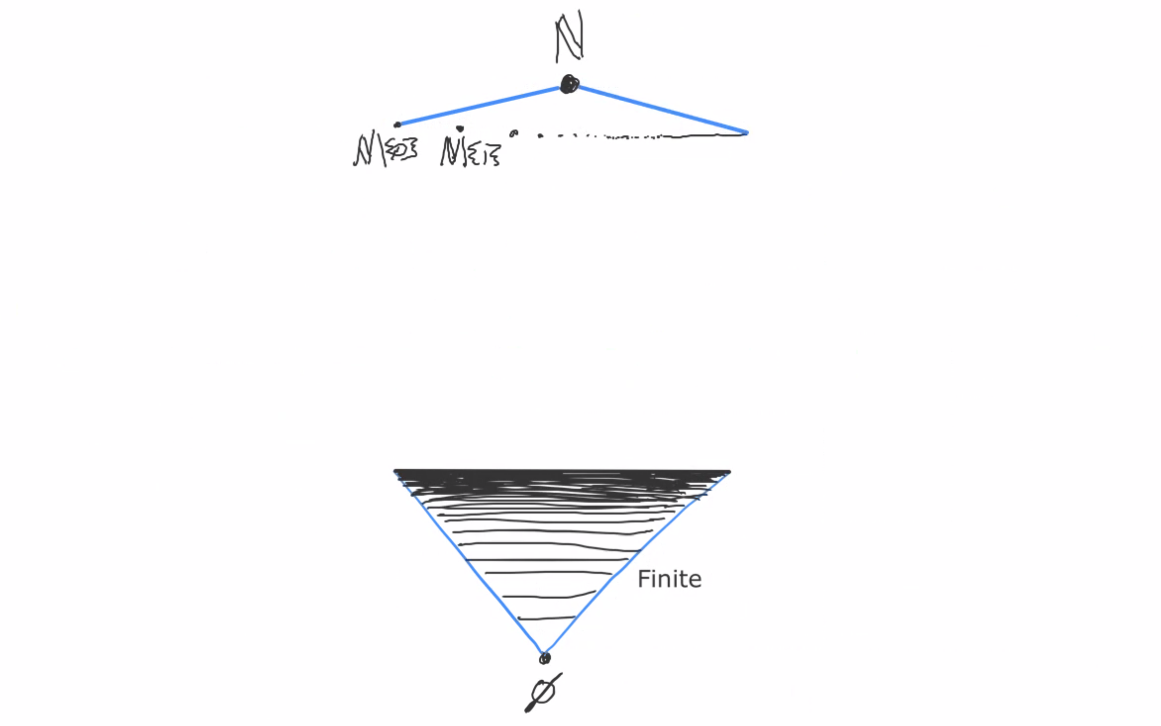
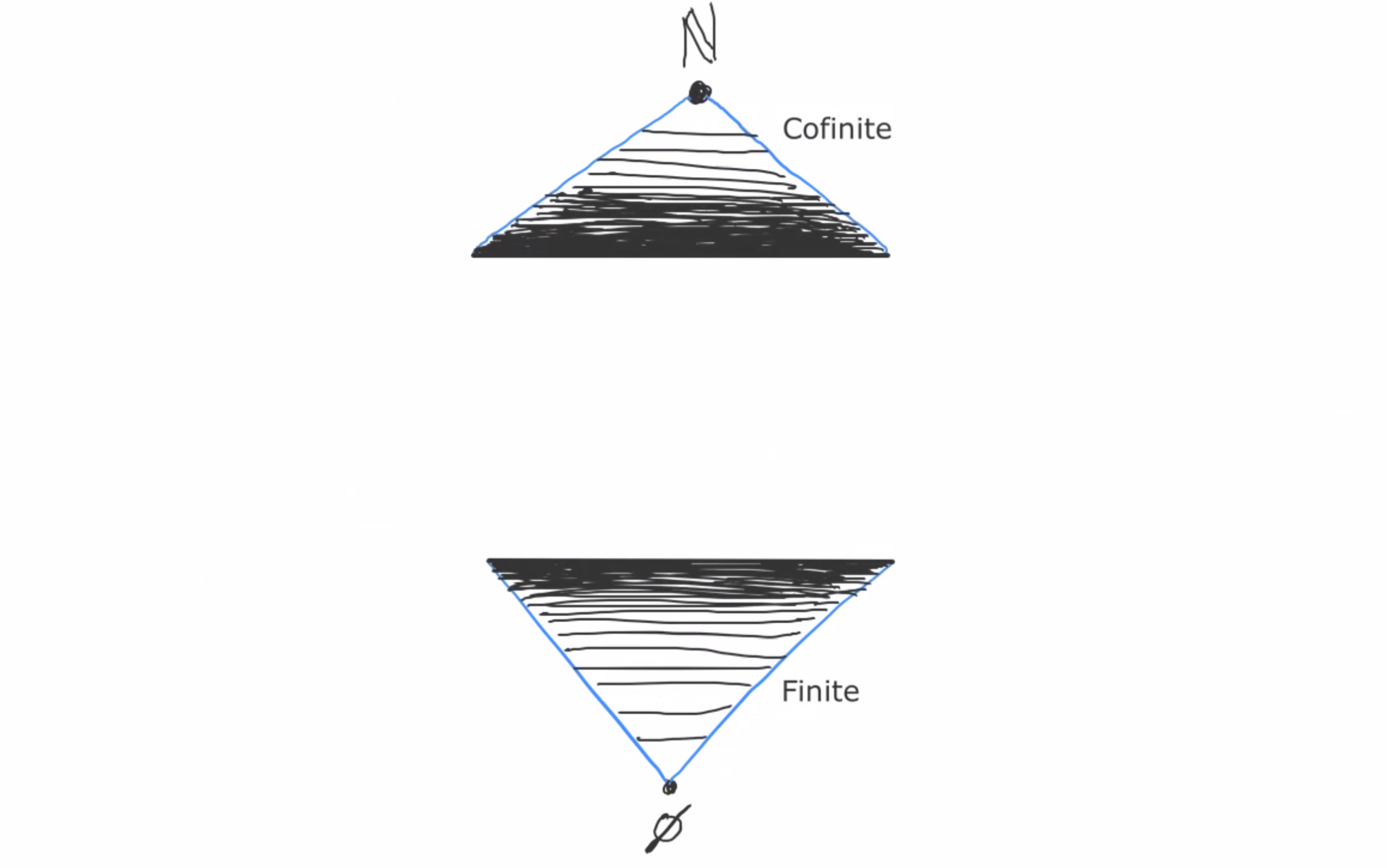
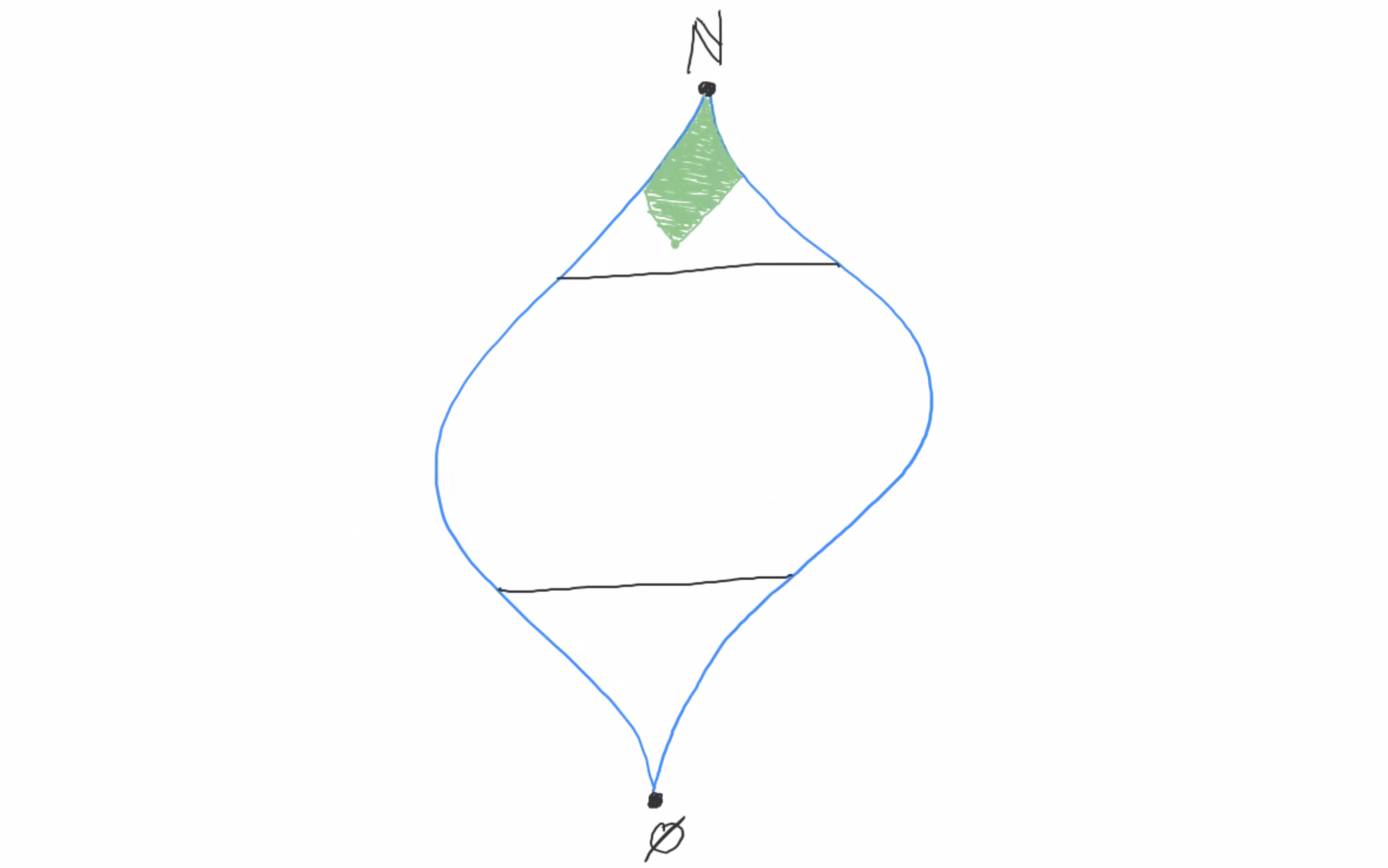
(4) We want to construct an equivalence relation on this set. We do so by first defining a free ultrafilter U on I. From the previous post, we know that every infinite set has a free ultrafilter on it, so as long as our index set is infinite, then we’re good to go.

With U in hand, we define the equivalence relation on Π(Mi)i∈I:

Let f and g be sequences (f,g: I → U(Mi)i∈I).
Then f ~ g if and only if { i ∈ I | f(i) = g(i) } ∈ U

You might be getting major deja-vu from the last post. Two sequences are said to be equivalent if the set of places-of-agreement is a member of the chosen ultrafilter. Since every free ultrafilter contains all cofinite sets, any two sequences that agree in all but finitely many places will be equivalent.

(5) Now all the pieces are in place. The ultraproduct of (Mi)i∈I with respect to U is the set of equivalence classes of Π(Mi)i∈I with respect to ~. This is typically written Π(Mi)i∈I/U. For a sequence a: I → U(Mi)i∈I we’ll denote the equivalence class it belongs to as [a].

Now, it’s not necessary for our indexed sequence (Mi)i∈I of L-structures to all be distinct. In fact, all the models can be the same, in which case we have (Mi)i∈I = (M)i∈I, and the ultraproduct Π(M)i∈I/U is called an ultrapower. The ultrapower of M with index set I and ultrafilter U can be written compactly as MI/U.

Some examples: The hypernaturals are the ultrapower ℕ/U = Π(ℕ)i∈ℕ/U where U is any free ultrafilter over ℕ. Similarly, the hyperreals are ℝ/U = Π(ℝ)i∈ℕ/U. The hyperintegers are ℤ/U. And so on.

(6) So far we’ve just defined the ultraproduct as a set (the set of equivalence classes of I-indexed sequences of elements from the models (Mi)i∈I). But we want the ultraproduct to have all the same structure as the models that we used as input. In other words, the ultraproduct of a bunch of L-structures will itself be an L-structure. To make this happen, we need to specify how the relation symbols and function symbols of L work in the ultraproduct model.

Here’s how it works. If f is a unary function symbol in the language L, then we define f on Π(Mi)i∈I/U by applying the function elementwise to the sequences. So:

f: Π(Mi)i∈I/U → Π(Mi)i∈I/U is defined as f([a])(i) = f(a(i)) for every i ∈ I.

What if f is a binary function symbol? Then:

f: (Π(Mi)i∈I/U)2 → Π(Mi)i∈I/U is defined as f([a], [b])(i) = f(a(i), b(i)) for every i ∈ I.

This generalizes in the obvious way to trinary function symbols, quaternary function symbols, and so on.

What about relations? Suppose R is a unary relation symbol in the language L. We need to define R on the ultraproduct Π(Mi)i∈I/U, and we do it as follows:

Π(Mi)i∈I/U ⊨ R([a]) if and only if { i ∈ I | Mi ⊨ R(a(i)) } ∈ U.

In other words, Π(Mi)i∈I/U affirms R([a]) if and only if the set of indices i such that Mi affirms R(a(i)) is in the ultrafilter. For example, if R holds for cofinitely many members of the sequence a, then R holds of [a].

If R is binary, we define it as follows:

Π(Mi)i∈I/U ⊨ R([a], [b]) if and only if { i ∈ I | Mi ⊨ R(a(i), b(i)) } ∈ U.

And again, this generalizes in the obvious way.

This fully defines the ultraproduct Π(Mi)i∈I/U as an L-structure! (If you’re thinking ‘what about constant symbols?’, remember that constants are just 0-ary functions)

Say that again, slower

That was really abstract, so let’s go through it again with the (hopefully now-familiar) example of the hypernaturals.

We start by defining an index set I. We choose I = ℕ.

Now define the language we’ll use. This will be the standard language of Peano arithmetic: one constant symbol (0), one relation symbol (<), and three function symbols (S, +, ×).

The family of structures in this language that we’ll consider (Mi)i∈I will just be a single structure repeated: for each i, Mi will be the L-structure ℕ (the natural numbers with 0, <, +, and × defined on it). So our family of structures is just (ℕ)i∈ℕ = (ℕ, ℕ, ℕ, ℕ, …).

Our sequences are functions from I to U(Mi)i∈I such that for each i∈I, f(i) ∈ Mi. For the hypernaturals, I and U(ℕ)i∈ℕ are both just ℕ, so our sequences are functions from ℕ to ℕ. We can represent the function f: ℕ → ℕ in the familiar way: (f(0), f(1), f(2), f(3), …).

The set of all sequences is the set of all functions from ℕ to ℕ. This is the direct product Π(ℕ)i∈ℕ = ℕ.

Now, we take any ultrafilter on I = ℕ. Call it U. We use U to define the equivalence relation on the direct product ℕ:

(a(0), a(1), a(2), …) ~ (b(0), b(1), b(2), …) if and only if { i ∈ ℕ | a(i) = b(i) } ∈ U

And taking equivalence classes of this relation, we’ve recovered our original definition of the hypernatural numbers! ℕ/U = *ℕ. Now we finish up by defining all functions and relations on *ℕ.

Functions are defined pointwise:

0 = [0, 0, 0, 0, …]
S[a(0), a(1), a(2), …] = [Sa(0), Sa(1), Sa(2), …]
[a(0), a(1), a(2), …] + [b(0), b(1), b(2), …] = [a(0) + b(0), a(1) + b(1), a(2) + b(2), …]
[a(0), a(1), a(2), …] ⋅ [b(0), b(1), b(2), …] = [a(0) ⋅ b(0), a(1) ⋅ b(1), a(2) ⋅ b(2), …]

We just have one relation symbol <, and relations are defined according to the ultrafilter:

[a(0), a(1), a(2), …] < [b(0), b(1), b(2), …] iff { i ∈ ℕ | ℕ ⊨ (a(i) < b(i)) } ∈ U

And we’re done!

Łoś’s theorem

Now we’re ready to prove Łoś’s theorem in its full generality. First, let’s state the result:

Fix any index set I, any language L, and any family of L-structures (Mi)i∈I. Choose a free ultrafilter U on I and construct the ultraproduct structure Π(Mi)i∈I/U. Łoś’s theorem says:

For every L-sentence φ, Π(Mi)i∈I/U ⊨ φ if and only if { i ∈ I | Mi ⊨ φ } ∈ U.

A special case of this is where our ultraproduct is an ultrapower of M, in which case it reduces to:

For every L-sentence φ, MI/U ⊨ φ if and only if M ⊨ φ

In other words, any ultrapower of M is elementary equivalent to M!

The proof is by induction on the set of all L-formulas.

Base case: φ is atomic

Atomic sentences are either of the form R(t1, …, tn) or (t1 = t2) for an n-ary relation symbol R and terms t1, … tn.

Suppose φ is R(t1, …, tn). This case is easy: it was literally the way we defined the interpretation of relation symbols in the ultraproduct model that Π(Mi)i∈I/U ⊨ R(t1, …, tn) if and only if {i ∈ I | Mi ⊨ R(t1, …, tn)} ∈ U.

Suppose φ is (t1 = t2). t1 and t2 are terms, so the ultraproduct model (Π(Mi)i∈I/U) interprets them as I-sequences, i.e. functions from I to U(Mi)i∈I such that t1(i) and t2(i) are both in Mi. We’ll write the denotations of t1 and t2 as [t1] and [t2]. Now, [t1] = [t2] iff { i ∈ I | t1 = t2 } ∈ U iff { i ∈ I | Mi ⊨ (t1 = t2) } ∈ U, which is what we want.

Inductive step: φ is ¬ψ, ψ∧θ, or ∃x ψ

Assume that Los’s theorem holds for ψ and θ. Now we must show that it holds for φ

Suppose φ is ¬ψ.

Then Π(Mi)i∈I/U ⊨ φ
iff Π(Mi)i∈I/U ⊭ ψ
iff { i ∈ I | Mi ⊨ ψ } ∉ U (by the inductive hypothesis)
iff { i ∈ I | Mi ⊨ ψ }c ∈ U (by the ultra property of U)
iff { i ∈ I | Mi ⊭ ψ } ∈ U

iff { i ∈ I | Mi ⊨ ¬ψ } ∈ U
iff { i ∈ I | Mi ⊨ φ } ∈ U

Suppose φ is ψ∧θ.

Then Π(Mi)i∈I/U ⊨ φ
iff Π(Mi)i∈I/U ⊨ ψ and Π(Mi)i∈I/U ⊨ θ
iff { i ∈ I | Mi ⊨ ψ } ∈ U and { i ∈ I | Mi ⊨ θ } ∈ U (by the inductive hypothesis)
iff { i ∈ I | Mi ⊨ ψ } ⋂ { i ∈ I | Mi ⊨ θ } ∈ U (by closure-under- of U)
iff { i ∈ I | Mi ⊨ ψ and Mi ⊨ θ } ∈ U
iff { i ∈ I | Mi ⊨ ψ∧θ } ∈ U
iff { i ∈ I | Mi ⊨ φ } ∈ U

Suppose φ is ∃x ψ.

Then Π(Mi)i∈I/U ⊨ φ
iff Π(Mi)i∈I/U ⊨ ∃x ψ
iff Π(Mi)i∈I/U ⊨ ψ(a) for some [a] ∈ Π(Mi)i∈I/U
iff { i ∈ I | Mi ⊨ ψ(a(i)) } ∈ U (by the inductive hypothesis)
iff { i ∈ I | Mi ⊨ ∃x ψ(x) } ∈ U

And that completes the proof! We don’t need to consider ∨, →, ↔, or ∀, because these can all be defined in terms of ¬, ∧, and ∃.

Now we know that the first-order properties of ultraproducts are tied closely to those of their component structures. The ultraproduct of any collection of two-element structures is itself a two-element structure. Same with the ultraproduct of any collection of structures, cofinitely many of which are two-element structures!

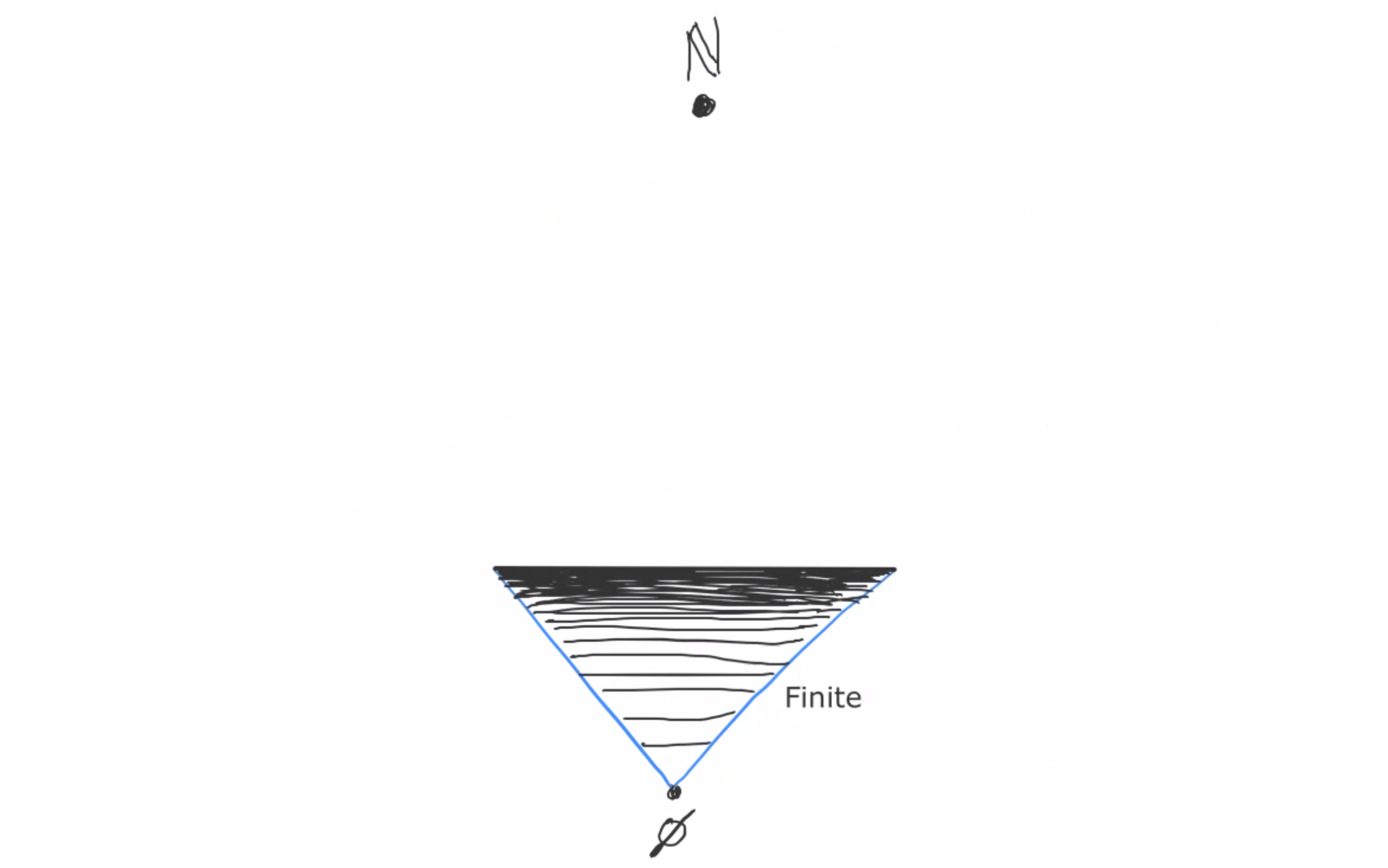
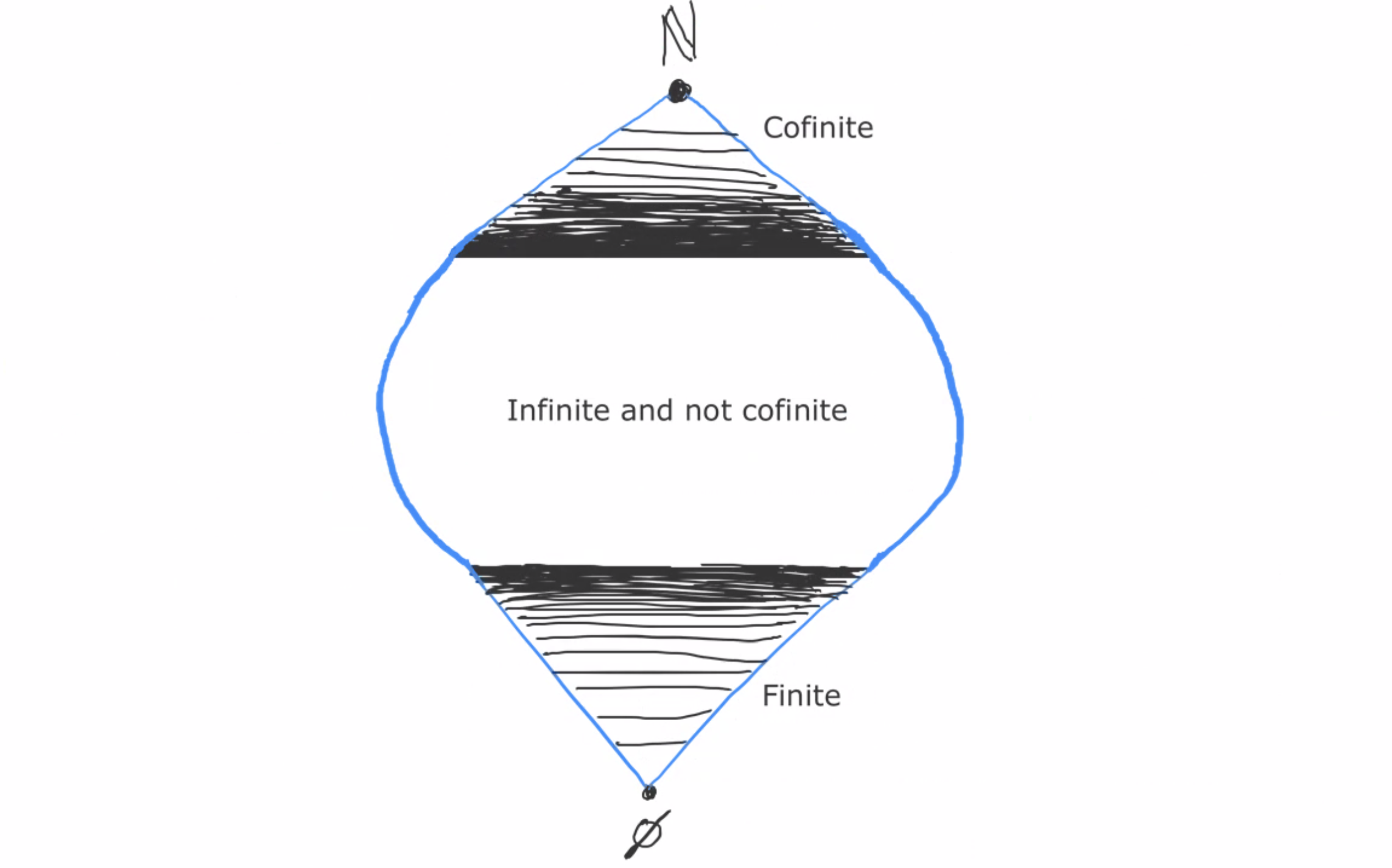
The ultraproduct of any collection of PA models is itself a PA model. The ultraproduct of any collection of groups is itself a group. But the ultraproduct of all finite groups need not itself be finite, because “I am finite” isn’t first-order expressible.

And in particular, an ultrapower of a structure M perfectly mimics ALL of the first-order properties of M!

Łoś’s theorem is an incredibly powerful tool we can wield to illuminate the strange structure of the hypernatural numbers. We’re now positioned to discover nonstandard prime numbers, infinitely even numbers, numbers that are divisible by every standard natural number, and infinitely large prime gaps. All of this (and more) in the next post!

Next: Weird nonstandard numbers

Hypernaturals in all their glory (Ultra Series 3)

Previous: Hypernaturals simplified

What is an ultrafilter? (with pretty pictures)

To define an ultrafilter we need to first define a filter. Here’s a pretty good initial intuition for what a filter is: a filter on a set X is a criterion for deciding which subsets of X are “large”. In other words, a filter provides us one way of conceptualizing the idea of large and small subsets, and it allows us to do so in a way that gives us more resolution than the cardinality approach (namely, assess size of sets just in terms of their cardinality). For example, in a countably infinite set X, the cofinite subsets of X (those that contain all but finitely many elements of X) have the same cardinality as the subsets of X that are infinite but not cofinite. But there’s some intuitive sense in which a set that contains all but finitely many things is larger than a set that leaves out infinitely many things. Filters allow us to capture this distinction.

Alright, so given a set X, a filter F on X is a collection of subsets of X (i.e. it’s a subset of 𝒫(X)) that satisfies the following four conditions:

(i) X ∈ F … “X is large”
(ii) ∅ ∉ F … “the empty set is not large”
(iii) If A ⊆ B and A ∈ F, then B ∈ F … “supersets of large sets are large”
(iv) If A ∈ F and B ∈ F, then A ⋂ B ∈ F … “intersections of large sets are large”

In other words, a filter on X is a set of subsets of X that contains X, doesn’t contain the empty set, and is closed under supersets and intersection. Note that a filter is also closed under union, because of (iii) (the union of A and B is a superset of A).

An ultrafilter is a filter with one more constraint, namely that for any subset of X, either that subset or its complement is in the filter.

(v) For any A ⊆ X, either A ∈ F or (X\A) ∈ F … “a set is either large, or if not, then its complement is large”

There’s a nice way to visualize filters and ultrafilters that uses the Hasse diagram of the power set of X. For a concrete example, let X = {a, b}. We can draw the power-set of X as follows:

We draw an arrow from A to B when A is a subset of B. Now, what are the possible filters on X? There are three, see if you can find them all before reading on.

Only two of these are ultrafilters. Which two?

Remember that for an ultrafilter U, every subset or its complement is in U. So an ultrafilter always contains half of all subsets. This gives an easy way to rule out the first one.

Another example: let X = {a, b, c}. Then the power-set of X looks like:

Note that we’ve left out some arrows, like the arrow from {a} to {a,b,c}. This is okay, because transitivity of the subset relation makes this arrow redundant. Anyway, what are some filters on X? Here are three of them:

Only one of these is an ultrafilter! You should be able to identify it pretty easily. See if you can pick out the other four filters, and identify which of them are ultrafilters (there should be two). And another exercise: why is the following not a filter?

Does it have any extension that’s an ultrafilter?

One thing to notice is that in all of these examples, when something is in the filter then everything it points to is also in the filter. This corresponds to ultrafilters being closed under supersets. Also, for any two things in the filter, their meet (their greatest lower bound; the highest set on the diagram that points to both of them) is also is the filter. This corresponds to closure under intersections.

Imagine that there is a stream flowing up the Hasse diagram through all the various paths represented by arrows. Choose any point on the diagram and imagine dripping green dye into the water at that point. The green color filters up through the diagram until it reaches the top. And everything that’s colored green is in the filter! This captures the idea that filters are closed under superset, but what about intersection? If X is finite, this corresponds to the dye all coming from a single source, rather than it being dripped in at multiple distinct points. The infinite case is a little trickier, as we’ll see shortly.

One other important thing to notice is that whenever we had an ultrafilter, it always contained a singleton. An ultrafilter that contains a singleton is called a principal ultrafilter, and an ultrafilter that doesn’t contain any singletons is called a free ultrafilter. So far we haven’t seen any free ultrafilters, and in fact as long as X is finite, any ultrafilter on X will be principal. (Prove this!) But the situation changes when X is an infinite set.

The Hasse diagram for an infinite set is a bit harder to visualize, since now we have uncountably many subsets. But let’s try anyway! What does the Hasse diagram of ℕ look like? Well, we know that ∅ is at the bottom and ℕ is at the top, so let’s start there.

Next we can draw all the singleton sets. ∅ points at all of these, so we’re not going to bother drawing each individual arrow.

Next we have all the pair sets, and then the triples. Each singleton points at infinitely many pairs, and each pair points at infinitely many triples.

And so on through all finite cardinalities.

Now what? We’ve only exhausted all the finite sets. We can now start from the top with the cofinite sets, those that are missing only finitely many things. First we have the sets that contain all but a single natural number:

Then the sets containing all but a pair of naturals, and so on through all the cofinite sets.

But we’re not done yet. We haven’t exhausted all of the subsets of ℕ; for instance the set of even numbers is neither finite nor cofinite. In fact, there are only countably many finite and cofinite sets, but there are uncountably many subsets of ℕ, so there must be a thick intermediate section of infinite sets that are not cofinite (i.e. infinite sets with infinite complements).

A sanity check that this diagram makes sense: start with a finite set and then add elements until you have a cofinite set. Between the finite set and the cofinite set there’s always an intermediate set that’s infinite but not cofinite. This matches with our image: any path from the finite to the cofinite passes through the middle section.

Now, what would a filter on the naturals look like on this diagram? If our filter is principal, then we can still roughly sketch it the same way as before:

How about an ultrafilter? Depends on whether it’s principal or free. Any principal ultrafilter must look like the third image above; it must start at the “finite” section and filter upwards (remember that principal means that it contains a singleton).

Any principal ultrafilter on ℕ can be written as { A ⊆ ℕ | n ∈ A } for some n ∈ ℕ.

What about free ultrafilters? A free ultrafilter contains no singletons. This implies that it contains no finite set. See if you can come up with a proof, and only then read on to see mine.

Suppose that U is a free ultrafilter on X and contains some finite set F. U is free, so it contains no singletons. So for every a ∈ F, the singleton {a} ∉ U. By ultra, X\{a} ∈ U. By closure-under-finite-intersection, the intersection of {X\{a} | a ∈ F} is in U. So X\F ∈ U. But now we have F ∈ U and X\F ∈ U, and their intersection is ∅. So ∅ ∈ U, contradicting filter.

So a free ultrafilter must contain no finite sets, meaning that it contains all the cofinite sets. Since it’s ultra, it also contains “half” of all the intermediate sets. So visually it’ll look something like:

That’s what a free ultrafilter on the naturals would look like if such a thing existed. But how do we know that any such object actually does exist? This is not so trivial, and in fact the proof of existence uses the axiom of choice. Here’s a short proof using Zorn’s Lemma (which is equivalent to choice in ZF).

Let F be any filter on X. Consider the set Ω of all filters on X that extend F. (Ω, ⊆) is a partially ordered set, and for any nonempty chain of filters C ⊆ Ω, the union of C is itself a filter on X. (Prove this!) The union of C is also an upper bound on C, meaning that every nonempty chain of filters has an upper bound. Now we apply Zorn’s Lemma to conclude that there’s a maximal filter U in Ω. Maximality of U means that U is not a subset of V for any V ∈ Ω.

Almost done! U is maximal, but is it an ultrafilter? Suppose not. Then there’s some A in X such that A ∉ U and (X\A) ∉ U. Simply extend U by adding in A and all supersets and intersections. This is a filter that extends F and contains U, contradicting maximality. So U is an ultrafilter on X!

Now, F was a totally arbitrary filter. So we’ve shown that every filter on X has an ultrafilter extension. Now let X be infinite and take the filter on X consisting of all cofinite subsets of X (this is called the Fréchet filter). Any ultrafilter extension of the Fréchet filter also contains all cofinite subsets of X, and thus contains no singletons. So it’s free! Thus any infinite set has a free ultrafilter.

Hypernatural numbers

Still with me? Good! Then you’re ready for the full definition of the hypernatural numbers, using ultrafilters. Take any free ultrafilter U on ℕ. U contains all cofinite sets and no finite sets, and is also decisive on all the intermediate sets. If you remember from the last post, this makes U a perfect fit for our desired “decisiveness criterion”.

Now consider the set of all countable sequences of natural numbers. Define the equivalence relation ~ on this set as follows:

(a1, a2, a3, …) ~ (b1, b2, b3, …) iff { k ∈ ℕ | ak = bk } ∈ U

Note the resemblance to our definition last post:

(a1, a2, a3, …) ~ (b1, b2, b3, …) iff { k ∈ ℕ | ak = bk } is cofinite

This previous definition corresponded to using the Fréchet filter for our criterion. But since it was not an ultrafilter, it didn’t suffice. Now, with an ultrafilter in hand, we get decisiveness!

Addition and multiplication on the hypernaturals is defined very easily:

[a1, a2, a3, …] + [b1, b2, b3, …] = [a1+b1, a2+b2, a3+b3, …]
[a1, a2, a3, …] ⋅ [b1, b2, b3, …] = [a1⋅b1, a2⋅b2, a3⋅b3, …]

Let’s now define < on the hypernaturals.

(a1, a2, a3, …) < (b1, b2, b3, …) if { k ∈ ℕ | ak < bk } ∈ U

The proof of transitivity in the previous post still works here. Now let’s prove that < is a total order.

Consider the following three sets:

X = { k ∈ ℕ | ak < bk }
Y = { k ∈ ℕ | ak > bk }
Z = { k ∈ ℕ | ak = bk }

The intersection of any pair of these sets is empty, meaning that at most one of them is in U. Could none of them be in U? Suppose X, Y, and Z are not in U. Then ℕ\X and ℕ\Y are in U. So (ℕ\X) ⋃ (ℕ\Y) is in U as well. But (ℕ\X) ⋃ (ℕ\Y) = Z! So Z is in U, contradicting our assumption.

So exactly one of these three sets is in U, meaning that a < b or b < a or a = b. This proves that using an ultrafilter really has fixed the problem we ran into previously. This problem was that the hypernaturals were quite different from the naturals in undesirable ways (like < not being a total order). The natural question to ask now is “Just how similar are the hypernaturals to the naturals?”

The answer is remarkable. It turns out that there are no first-order expressible differences between the naturals and the hypernaturals! Any first-order sentence that holds true of the natural numbers also holds true of the hypernatural numbers! This result is actually just one special case of an incredibly general result called Łoś’s theorem. And in the next post we are going to prove it!

Next up: Łoś’s theorem and ultraproducts!

Hypernaturals Simplified (Ultra Series 2)

Previous: Introduction

What is a hypernatural number? It is a collection of infinitely long sequences of natural numbers. More precisely, it is an equivalence class of these infinite sequences.

An equivalence class under what equivalence relation? This is a little tricky to describe.

I’ll start with a slight lie to simplify the story. When we see the trouble that results from our simple definition, I will reveal the true nature of the equivalence relation that gives the hypernaturals. In the process you’ll see how the notion of an ultrafilter naturally arises.

So, hypernaturals are all about infinite sequences of natural numbers. Some examples of these:

(0,1,2,3,4,5,6,7,8,9,…)
(0,1,0,2,0,3,0,4,0,5,…)
(1,2,1,2,1,2,1,2,1,2,…)
(0,2,4,6,8,10,12,14,…)
(3,1,4,1,5,9,2,6,5,3,…)

We’ll define an equivalence relation ~ between sequences as follows:

Let x and y be infinite sequences of natural numbers.
Then x ~ y iff x and y agree in all but finitely many places.

For example, (0,1,2,3,4,5,6,…) ~ (19,1,2,3,4,5,6,…), because these two sequences only disagree at one spot (the zero index).

(1,1,2,2,4,4,…) and (1,2,4,8,…) are not equivalent, because these sequences disagree at infinitely many indices (every index besides the zeroth index).

Same with (0,1,2,3,4,5,6,…) and (1,2,3,4,5,6,7,…); even though they look similar, these sequences disagree everywhere.

(2,4,6,8,10,12,14,…) and (2,0,6,0,10,0,14,…) are not equivalent, because these sequences disagree at infinitely many indices (every odd index).

One can easily check that ~ is an equivalence relation, and thus it partitions the set of sequences of naturals into equivalence classes. We’ll denote the equivalence class of the sequence (a1, a2, a3, …) as [a1, a2, a3, …]. These equivalence classes are (our first stab at the definition of) the hypernaturals!

For instance, the equivalence class of (0,0,0,0,0,…) contains (1,4,2,0,0,0,0,0,…), as well as (0,2,4,19,0,0,0,0,…), and every other sequence that eventually agrees with (0,0,0,0,…) forever. So all of these correspond to the same hypernatural number: [0,0,0,0,…]. This object is our first hypernatural number! It is in fact the hypernatural number that corresponds exactly to the ordinary natural number 0. In other words 0 = [0,0,0,0,…].

[1,1,1,1,…] is a distinct equivalence class from [0,0,0,0,…]. After all, the sequences (0,0,0,0,…) and (1,1,1,1,…) disagree everywhere. You might guess that [1,1,1,1,…] is the hypernatural analogue to the natural number 1, and you’d be right!

For any standard natural number N, the corresponding hypernatural number is [N,N,N,N,N,…], the equivalence class of the sequence consisting entirely of Ns.

Now consider the hypernatural [0,1,2,3,4,5,6,…]. Let’s call it K. Does K = N for any standard natural number N? In other words, is (0,1,2,3,4,5,6,…) ~ (N,N,N,N,N,…) true for any finite N? No! Whatever N you choose, it will only agree with (0,1,2,3,4,5,6,…) at one location. We need cofinite agreement, and here we have merely finite agreement. Not good enough! This means that K is our first nonstandard natural number!

How does K relate to the standard naturals in terms of order? We haven’t talked about how to define < on the hypernaturals yet, but it’s much the same as our definition of =.

[a1, a2, a3, …] = [b1, b2, b3, …]
iff
{ k∈ℕ | ak = bk } is cofinite

[a1, a2, a3, …] < [b1, b2, b3, …]
iff
{ k∈ℕ | ak < bk } is cofinite

Exercise: Verify that this is in fact a well-defined relation. Every equivalence class has many different possible representatives; why does the choice of representatives not matter for the purpose of describing order?

Now we can see that K > N for every standard N. Look at (0,1,2,3,4,5,…) and (N,N,N,N,…). The elements of the first sequence are only less than the elements of the second sequence at the first N indices. Then the elements of K are greater than the elements of N forever. So elements of K’s representative sequence are greater than elements of N’s representative sequence in a cofinite set of indices. Thus, K > N for every standard N. So K is an infinitely large number!

Here’s another one: K’ = [0,2,4,6,8,…]. You can see that K’ > K, because the elements of K’ are greater than those of K at all but one index (the first one). So we have another, bigger, infinite number.

Addition and multiplication are defined elementwise, so

K + K
= [0,1,2,3,4,…] + [0,1,2,3,4,…]
= [0+0, 1+1, 2+2, 3+3, 4+4, …]
= [0,2,4,6,8,…]
= K’

K’
= [0,2,4,6,8,…]
= [2⋅0, 2⋅1, 2⋅2, 2⋅3, 2⋅4, …]
= 2⋅[0,1,2,3,4,…]
= 2⋅K

Predictably, we get many many infinities. In fact, there are continuum many nonstandard hypernatural numbers!

Proof: we construct an injection f from ℝ to *ℕ. If x is a real number, then f(x) := [floor(x), floor(10x), floor(100x), floor(1000x), …]. For example, f(35.23957…) = [35,352,3523,35239,352395, …]. For any two distinct reals x and y, the sequences x and y will eventually disagree forever. So each real is mapped to a distinct hypernatural, meaning that there are no more reals than hypernaturals. At the same time, there are no more hypernaturals than reals, because there are only continuum many countable sequences of natural numbers. So |*ℕ| = |ℝ|.

It turns out that every nonstandard hypernatural number is also larger than every standard natural number. We’ll see why in a bit, but it’ll take a bit of subtlety that I’ve yet to introduce.

Now, > is transitive in ℕ. Is it also transitive in *ℕ? Yes! Suppose A > B and B > C. Choose any representative sequences (a1, a2, a3, …), (b1, b2, b3, …), and (c1, c2, c3, …) for A, B, and C. Then X = { k∈ℕ | ak > bk } and Y = { k∈ℕ | bk > ck } are both cofinite. The intersection of cofinite sets is also cofinite, meaning that X⋂Y = { k∈ℕ | ak > bk and bk > ck } ⊆ { k∈ℕ | ak > ck } is cofinite. So A > C!

It’s a good sign that > is transitive. But unfortunately, the story I’ve told you thus far starts to break down here. The greater-than relation is a total order on the natural numbers. For any naturals a and b, exactly one of the following is true: a = b, a > b, b > a. But this is not true of the hypernaturals!

Consider the two hypernatural numbers n = [0,1,0,1,0,1,…] and m = [1,0,1,0,1,0,…]. Are n and m equal? Clearly not; they disagree everywhere. So n ≠ m.

Is n > m? No. The set of indices where n’s sequence is greater than m’s sequence is {1, 3, 5, 7, …}, which is not cofinite.

So is m > n? No! The set of indices where m’s sequence is greater than n’s sequence is {0, 2, 4, 6, …}, which is also not cofinite!

So as we’ve currently defined the hypernatural numbers, the > relation is not a total relation on them. This might be fine for some purposes, but we’ll be interested in defining the hypernaturals to mirror the properties of the naturals as closely as possible. So we’ll have to tweak our definition of the hypernaturals. The tweak will occur way back at the start where we defined our equivalence relation on sequences of naturals.

Recall: we said that two sequences (a1, a2, a3, …) and (b1, b2, b3, …), are equivalent if they agree in all but finitely many places. Said another way: a ~ b if { k∈ℕ | ak = bk } is cofinite. We defined > similarly: a > b if the agreement set for > is cofinite.

The problem with this definition was that it wasn’t definitive enough. There are cases where the agreement set is neither cofinite nor finite. (Like in our previous example, where the agreement set was the evens.) In such cases, our system gives us no direction as to whether a > b or b > a. We need a criterion that still deals with all the cofinite and finite cases appropriately, but also gives us a definitive answer in every other case. In other words, for ANY possible set X of indices of agreement, either X or X’s complement must be considered “large enough” to decide in its favor.

For example, maybe we say that if { k∈ℕ | ak = bk } = {0,2,4,6,8,…}, then a > b. Now our criterion for whether a > b is: the set of indices for which ak = bk is either cofinite OR it’s the evens. This implies that [1,0,1,0,1,0,…] > [0,1,0,1,0,1,…].

Once we’ve made this choice, consistency forces us to also accept other sets besides the evens as decisive. For instance, now compare (0,0,1,0,1,0,…) and (0,1,0,1,0,1,…). The set of indices where the first is greater than the second is {2,4,6,8,…}. But notice that the first differs only cofinitely from (1,0,1,0,…), meaning that [0,0,1,0,1,0,…] = [1,0,1,0,1,0,…]. The conclusion is that [0,0,1,0,1,0,…] > [0,1,0,1,0,1,…], which says that the set of indices {2,4,6,8,…} must also be decisive. And in general, once we’ve accepted the evens as a decisive set of indices, we must also accept the evens minus any finite set.

The three criterion we’ve seen as desirable for what sets of indices will count as decisive are (1) includes all cofinite sets, (2) for any set X, either X or X’s complement is decisive, and (3) consistency. These requirements turn out to correspond perfectly to a type of mathematical object called a free ultra-filter!

In the next post, we will define ultrafilters and finalize our definition of the hypernatural numbers!

Ultrafilters, Ultraproducts, and Hypernaturals 1: Introduction

This is the series I wish would have existed a month ago when I first started learning about ultrafilters and ultraproducts. First of all, what’s the motivation for learning about these ultra-objects? I imagine that if you’re here, you probably already have some degree of interest in ultrafilters, ultraproducts, or nonstandard models of arithmetic. But I’ll see if I can bolster that interest a little bit.

The most exciting application to me personally is that ultraproducts give you a recipe for constructing new mathematical structures out of familiar ones. Out of some model M one can construct a a new model *M, which typically has a much richer and stranger structure, but is nonetheless elementarily equivalent to M (this is called Łoś’s theorem). Elementary equivalence means that all the expressive resources of first-order logic are insufficient to tell M and *M apart: they agree on all first-order sentences.

For example, the ultraproduct of ℝ (the real numbers) is *ℝ, the hyperreal numbers. The hyperreals contain an enormous supply of infinitesimal quantities clustered around every real, as well as infinitely large quantities. And all the usual operations on ℝ, like addition and multiplication, are already nicely defined in *ℝ, meaning that these infinitesimals and infinities have a well-defined algebraic structure. And Łoś’s theorem tells us that ℝ and *ℝ are elementary equivalent: any first-order sentence true of the reals is also true of the hyperreals.

Another example: the ultraproduct of ℕ (the natural numbers) is *ℕ, the hypernaturals. The hypernaturals don’t contain any infinitesimals, but they do contain an uncountable infinity of infinite numbers. And since *N and N are elementarily equivalent, *ℕ is a model of true arithmetic! This is super exciting to me. True arithmetic is this unimaginably complicated set of sentences; there’s no Turing machine that decides which sentences reside in true arithmetic, nor is there a Turing machine with a halting oracle that does the job, nor even a Turing machine with a halting oracle for Turing machines with halting oracles! The computational complexity of true arithmetic is the limit of this sequence of progressively harder halting problems: you can only decide the set if you have an oracle for the halting problem, plus an oracle for the halting problem for TMs with oracles for the halting problem, plus an oracle for the halting problem for TMs with oracles for the halting problem for TMs with oracles for the halting problem, and so on. This level of complexity is known as 0(ω).

So true arithmetic is this impossibly uncomputable set of sentences. We know trivially that ℕ is a model of true arithmetic, because that’s how true arithmetic is defined { φ | ℕ ⊨ φ }. And we also know that true arithmetic has nonstandard models, because it’s a first-order theory and no first order theory can categorically define ℕ (I think the easiest way to see why this is true is to apply the Löwenheim-Skolem theorem, but – self-promotion alert – there’s also this very nice and simple proof from first principles). And ultraproducts allow us to construct an explicit example of one of these nonstandard models! You can actually write down some of these nonstandard numbers (they look like infinite sequences of natural numbers) and discover their strange properties. For example, (2, 3, 5, 7, 11, …) is a nonstandard prime number, (1, 2, 4, 8, 16, …) is infinitely even, and (0!, 1!, 2!, 3!, 4!, …) is a multiple of every standard natural number. We’ll dive into all of this soon enough.

Ultrafilters and ultraproducts also have applications outside of logic. A fairly basic result about ultrafilters (that every ultrafilter over a finite set contains a singleton) is equivalent to Arrow’s impossibility theorem in voting theory (that any voting system with unanimity, independence of irrelevant alternatives (IIR), and finitely many voters contains a dictator). And the existence of a singleton-free ultrafilter over an infinite set (a free ultrafilter) shows that with infinitely many voters, there’s a non-dictatorial voting system with unanimity and IIR. There’s a pretty good description of those results here, but finish reading my post first!

Nick Bostrom in an old paper titled Infinite Ethics describes how to apply ultrafilters to resolve some of the issues that arise when trying to apply utilitarian ethics in a universe with infinitely many experiencers. Suppose that the current universe contains an infinite number of experiencers, each of whom is having an experience with a valence of +1. By pressing a button, you can immediately transition to a universe where everybody is now experiencing a valence of +2. Clearly pressing the button is a utilitarian good. But 1+1+1+… = ∞ = 2+2+2+…. So it looks like a standard account of utility as real numbers says that the utility of the +2 world is the same as the utility of the +1 world (both just ∞). But if we treat utilities as hyperreal numbers instead of ordinary real numbers, then we can do the comparison and get the right answer. It’s worth noting that this approach doesn’t fix all the problems raised by an infinite universe; for instance, if pressing the button only increases a finite number of experiencers from valence +1 to valence +2, then the net utility of the universe is unchanged, even with hyperreal utilities. (This corresponds to a property that we’ll see soon, which is that a free ultrafilter contains no finite sets.)

Okay, introduction over. Hopefully you’re now excitedly asking yourself the question “So what are these ultrafilters and ultraproducts anyway??” The story begins in the next post!

Hypernaturals Simplified

Even Numbers are Tautologies

To each atomic proposition P assign a natural number p. If that natural number is even, then its corresponding proposition is true. If the number is odd then the proposition is false.

If you have two numbers n and m and you multiply them, the result is even so long as either n or m is even. So multiplication is like or; P∨Q corresponds to pq.

Negation is like adding 1: even becomes odd and odd becomes even. So ¬P corresponds to p+1.

Consider addition: p+q is even if p and q are both even or both odd. So p+q is like the biconditional ↔.

Other connectives can be formed out of these. Take P∧Q: P∧Q is equivalent to ¬(¬P∨¬Q), which is (p+1)(q+1) + 1. So P∧Q corresponds to pq+p+q+2. P→Q is ¬P∨Q, which is (p+1)q.

The logical constants ⊤ and ⊥ correspond to numerical constants: ⊤ can be assigned 0 and ⊥ assigned 1, for instance.

Tautologies translate to algebraic expressions which are always even. For instance, P→P translates to (p+1)p, which is always even. P→(Q→P) translates to (p+1)(q+1)p, which is also always even. P∨¬P translates to p(p+1), always even.

Contradictions translate to algebraic expressions which are always odd. P∧¬P translates to (p+1)(p+2) + 1, which is always odd. And so on.

Inference rules can be understood as saying: if all the premises are even, then the conclusion will be even. Take conjunction elimination: P∧Q ⊨ P. This says that if (p+1)(q+1) + 1 is even then p is even, which ends up being right if you work it out. Modus ponens: P, P→Q ⊨ Q. This says that if p and (p+1)q are both even, then q is even. Again works out!

You can also work the other way: For any number p, p(p+1) is even. Translating into propositional logic, this says that P∨¬P is a tautology. We’ve proved the law of the excluded middle! It’s interesting to note that earlier we saw that P→P translates to (p+1)p. So in some sense the law of the excluded middle is just self-implication but with the two products reversed!

First Order Truth Trees

The analytic tableaux (also called truth tree) style of proof system is really nice. The tree structure tends to resemble the actual process of mathematical reasoning better than the Hilbert-style linear proof systems, and I find that the formal proofs are much easier to follow. For first-order logic (without equality), the system involves four new inference rules to deal with quantifiers. There are a few different logically equivalent choices for these rules, but here is my favorite:

Universal instantiation ∀
∀x φ(x)

φ(t)
(where t is any closed term – any term without free variables)

Existential instantiation ∃
∃x φ(x)

φ(a)
(where a is any new constant)

Negated universal ¬∀
¬∀x φ

∃x ¬φ

Negated existential ¬∃
¬∃x φ

∀x ¬φ

The instantiation rules are actually quite interesting. Suppose that you’re working in the language of ZFC. ZFC has no constant or function symbols, only a single binary relation symbol: ∈, interpreted as “is an element of”. This seems to raise a problem for using the instantiation rules. For universal instantiation, we can only apply it to closed terms. But a language with no constants has no closed terms! And looking at existential instantiation, there’s a similar problem: we’re supposed to derive φ(a), where a is a new constant, but our language has no constants!

So what’s up? Does the standard first-order analytical tableaux approach not work for simple languages like ZFC? Insofar as ZFC is a shining beacon of what first-order logic can accomplish, this is a little disconcerting.

Actually, the instantiation rules work exactly as stated for ZFC. The subtlety in their interpretation is that when running proofs, you are allowed to (and in fact, often must) expand the language. So when you do existential instantiation, you don’t choose a constant symbol that already exists inside your language. Instead, you add a totally new constant symbol to your language, and then declare that φ holds of this symbol. Similarly, you can do universal instantiation in a language with no closed terms, simply by expanding the language to include some constants.

Now, if we’re expanding the language in the course of the proof, then who’s to say that in the end our proof will still be valid for our original language? Well, suppose we’re working in some minimal language L that has no constants. Let T be our background theory (the set of non-tautologies that we’re taking as assumptions). When we do existential instantiation, we always create a new constant. Let’s call it a. We then expand the language into L’ = L ⋃ {a}, and we expand our assumptions to T’ = T ⋃ {φ(a)}. When we do universal instantiation, we either use an existing closed term or create a new one. In the second case, we create a new constant b and form a new language L’ = L ⋃ {b}. We also expand our assumptions to a new set T’ = T ⋃ {φ(b)}.

The important thing to note is that we haven’t done anything that invalidates any models of T! If T originally contained a sentence of the form ∀x φ(x), then adding c and declaring φ(c) doesn’t conflict with this. And if T originally contained a sentence of the form ∃x φ(x), then in every model of T at least one thing satisfies φ. So when we add a new constant c, that constant can just refer back to any of these φ-satisfiers.

You might think: “But hold on! How can we be sure that it’s safe to just add new constants? Couldn’t we expand the domain too much, in a way that’s inconsistent with our original theory?” The answer to this is that the domain doesn’t have to expand to accommodate new constants! These constants can refer to existing elements of the domain. For instance, suppose T contains six existential statements and a sentence that says there are exactly five objects. Each time we run existential instantiation on one of the six existential sentences, we create a new constant. So we’ll get six new constants. But these constants can refer to the same value! And since our theory already says that there are five objects, the models of our expanded theory will also contain exactly five objects, meaning that in every model of our original theory, the new constants will refer to elements of the domain that already exist. No domain expansion!

Ok, but how do we know that there isn’t some very complicated sentence ψ that was originally true in every model of T, but becomes false in some models of T’? To fully prove that this never happens, we could do induction over all sentences in the language, showing that any sentence that is entailed by T is also entailed by T’. But considering the details of the expansion process, and trying to come up with ways that the expansion might fail, is a good way to get an intuition for why this proof system works.

I’ll close with a few examples of using analytic tableaux to prove basic results in PA and ZFC. Think of this as a proof of concept! (Each of these proofs also uses some rules regarding equality, which are obvious enough despite that I haven’t explicitly defined them).

First, we show that PA proves ∀x (0 + x = x). This is nontrivial, despite that ∀x (x + 0 = x) is an axiom!

Next, a proof from ZFC that the empty set exists and is unique:

Now a proof from PA that addition is commutative. This one is shockingly complicated for such a simple concept, and requires three uses of induction, but this goes to show how basic the axioms of PA really are! If you look closely, you’ll also notice that this proof replicates the proof of ∀x (0 + x = x) from above!

Final example, here’s a PA proof that no number is its own successor. This rules out nonstandard models of arithmetic with one nonstandard number!

One nonstandard is worth infinitely many standards

Suppose that M is a nonstandard model of true arithmetic (the set of all first-order sentences in the language of PA that are true in the standard model of arithmetic, ℕ). Now, take any formula φ(x) with one free variable. Suppose that there’s some nonstandard number k in M such that φ holds of k. Since k is larger than every standard natural, the following infinite set of sentences are all true in M:

∃x (x > 0 ∧ φ(x))
∃x (x > 1 ∧ φ(x))
∃x (x > 2 ∧ φ(x))

∃x (x > 1000000 ∧ φ(x))

Since M is a model of true arithmetic, and true arithmetic is complete (that is, each sentence or its negation appears in the theory), the standard model ℕ must also affirm all of these sentences. So it must be true of every standard natural that there’s a larger standard natural satisfying φ. In other words, you can guarantee that there are infinitely many standard naturals that satisfy a property φ, just by finding a single nonstandard number k that satisfies φ in a model of true arithmetic!

Furthermore, since in ℕ it is true that every standard natural has a larger standard natural satisfying φ, the sentence ∀x ∃y (y > x ∧ φ(y)) is true in ℕ. So this sentence must be true in every model of true arithmetic, including M! This means that just by finding a single nonstandard satisfying φ, you can immediately be sure that there are infinitely many standard numbers AND infinitely many nonstandard numbers (in every nonstandard model of TA!) satisfying φ. This is pretty dramatic!

As an example, consider the twin prime conjecture. We can construct the predicate isPrime(x) in first-order PA with the formula ∀y (∃z (y⋅z = x) → (y=1 ∨ y=x)). Then the predicate isTwinPrime(x) is just: isPrime(x) ∧ isPrime(x+2). Now the twin prime conjecture just says that ∀x ∃y (y > x ∧ isTwinPrime(y)), which is exactly the form we saw in the last paragraph! So to prove the twin prime conjecture, it suffices to demonstrate a single nonstandard twin prime in a model of true arithmetic.

This post is lying to you

In classical logic there are exactly two truth values, True and False, and every sentence has exactly one of these truth values. Consider the Liar sentence: “This sentence is false.” If this sentence is True, then it must be False. And if it’s False, then it must not be False. If we apply classical logic to this sentence, then it must have one of the two truth values. But whichever way we go, we find ourselves in trouble. And so the Liar sentence glitches out classical logic and produces an error.

But not so fast. For the Liar sentence to glitch out classical logic, it must first be the case that the sentence can actually be produced in classical logic. We start with an English sentence “This sentence is not true” and reason intuitively about what classical logic would do with this sentence, but we must be able to form this sentence in classical logic in order for classical logic to have anything to say about it.

There are two major hurdles with importing “This sentence is not true” into classical logic: translating “this sentence” and translating “is not true”. The first requires us to be able to have self-referential sentences. It’s not so obvious to see how we accomplish this with the machinery of classical logic. The second requires us to have a truth predicate. This perhaps seems prima facie easier to do, but it turns out that it has its own host of issues.

Let’s deal with the second issue first: how do we make sense of “is not true”? We’ll start by looking at “is true” (once we have this, then we can just negate it to get “is not true”). So, how do we make sense of “is true”?

When we say “X is true”, we aren’t assigning equality between an object X and an object True. We’re instead attributing the property of truthiness to the sentence X. So “is true” seems to act kind of like a predicate in first-order logic. But there’s a problem. Predicates apply to objects in the domain of a model, not to sentences in the language itself. For instance, the predicate “is red” might apply to firetrucks and Clifford, as objects in the universe, but it’s not going to apply to sentences in the language.

With this in mind, it appears that “is true” is actually more like a modal operator. It applies to sentences, not objects. We could introduce a modal operator T such that TX is interpreted as “X is true”, and add an axiom schema that says for every sentence φ, φ ↔ Tφ. The problem with this is that we will never get self reference with this approach. We want to create a sentence P that says “P is not true”. We could try something like P ↔ ¬TP, but this ends up just being a false sentence, not paradoxical. What’s missing is that the sentence “P ↔ ¬TP” is not equivalent to the sentence P: they’re just different sentences.

So the modal approach to interpreting “is true” has failed for our purposes. It’s simply not subtle enough to allow us to express self-reference. So let’s return to the predicate approach. The problem was that predicates apply to objects, not sentences. But what if the sentences were themselves objects? Of course, the sentences cannot literally be objects: they are purely syntactical items, whereas objects exist in the semantics (the interpretation of the language). But each sentence could have some sort of representative object in the domain.

What Gödel showed is that this is indeed possible. He designed a coding technique such that every sentence in the language gets assigned a particular natural number, and no two sentences have the same number. And if sentences correspond to numbers, then properties of those sentences can be translated into properties of those numbers!

Now if our language is sufficiently expressive to talk about natural number arithmetic, then our sentences can express properties of other sentences! In other words, we want a theory in a logic that has ℕ as a model. And we also want it to be sufficiently expressive to be able to talk about properties of numbers, like “being prime” or “being twice-divisible by 7”. Then we can imagine a predicate True(x), such that True(x) is True if and only if the sentence encoded by the number x is True.

For notational convenience, we’ll write “the number that encodes the sentence P” as ⟦P⟧. Then what we want of our truth predicate is that for every sentence φ, True(⟦φ⟧) ↔ φ.

Now, returning to the Liar sentence, we’ve dealt with “is true”, but now have to deal with “this sentence”. Remember that we want a sentence φ that asserts that the truth predicate does not apply to itself. In other words, we want φ to be the same thing as ¬True(⟦φ⟧). But how can this be? Clearly these are two different sentences, no?

Well, it’s not so obvious that φ and ¬True(⟦φ⟧) are actually distinct sentences. Remember that ⟦φ⟧ is just some number. So the sentence φ might be ¬True(9129828475651384). This is only a genuine liar sentence if 9129828475651384 encodes the sentence φ.

So really what we need to do is to look for some natural number n such that the sentence encoded by n is exactly “¬True(n)”. This would be a sentence which if true must be false, and if false must be true. It’s not at all obvious that such a natural number exists. But in 1934, Carnap proved the diagonal lemma, the tool necessary to construct such a number.

The diagonal lemma says that in any theory that can express natural number arithmetic (specifically, a theory that can define all primitive recursive functions), and for every predicate P(x), there’s a sentence ψ such that ψ ↔ P(⟦ψ⟧) is provable. Let P(x) be equal to ¬True(x), and we get that there’s a sentence ψ such that ψ ↔ ¬True(⟦ψ⟧) is provable!

In other words, there’s a sentence ψ encoded by a number n, such that ψ is true if and only if ¬True(n). This is exactly the liar paradox! We’ve succeeded at sneaking in a contradiction to classical logic! So what does this mean? Is classical logic ultimately all inconsistent? Do we need to rebuild logic from the ground up?

Not quite! Notice that to actually get to the point where we could express the Liar sentence, we had to take on a lot of assumptions. Let’s list them all out:

  1. Our language allows us to express natural number arithmetic.
  2. Our theory of natural numbers is strong enough to allow Gödel coding.
  3. Our theory of natural numbers is strong enough to express every primitive recursive function.
  4. There is a truth predicate.

From these assumptions, we were able to prove an inconsistency. But this doesn’t mean that classical logic is therefore inconsistent! Rather, it means that any consistent theory has to violate at least one of these assumptions! In particular, if we have a consistent theory that allows us to do both Gödel coding and to express primitive recursive functions, then this theory cannot have a truth predicate!

It’s important to understand that #4 here really is an assumption. When I described a truth predicate, I said “we can imagine that such a predicate exists.” I never showed you how to explicitly construct it! We could always explicitly add in a truth predicate T to a theory of arithmetic, and then assert as axioms φ ↔ T(⟦φ⟧) for every sentence φ. And the above line of reasoning shows us that doing so will render our theory inconsistent. If we don’t explicitly add in a truth predicate, then we could try to construct it from primitive relation and function symbols of the language. But the above line of reasoning shows us that no matter how hard we try, we will never succeed in this construction!

It’s interesting to note that (2) and (3) are actually different assumptions. (3) implies (2), but (2) doesn’t imply (3). In other words, you can have very weak theories of arithmetic that are expressive enough to do Gödel coding, but not expressive enough to prove the diagonal lemma! The amazing feature of these theories is that it’s possible for them to prove their own consistency without becoming inconsistent!

Finally, notice that the diagonal lemma was quite a bit more powerful than what we strictly required for our reasoning above. In particular, it allowed us to talk about ANY predicate whatsoever, not just a truth predicate. Consider what happens when instead of using “is true” as our predicate, we use “is provable”. You might get a somewhat interesting result!

Asymmetry between the infinite and finite

This is well-trod territory for this blog, but I want to give a little reminder of some of the subtleties involving infinity in logic. In particular, there’s a fun asymmetry between the finite and the infinite in terms of the expressive power of first order logic.

Consider the set of all first order sentences that are true in every infinite model. This includes any tautology (like P ∨ ¬ P), as well as some other sentences like ∃x ∃y (x ≠ y) (which says that there are at least two distinct things). Are there any finite models that satisfy this entire set of sentences?

Answer is no: for any finite n you can form a sentence that says “there are at least n things”. E.g. for n = 4 we say ∃x ∃y ∃z ∃w (x≠y ∧ x≠z ∧ x≠w ∧ y≠z ∧ y≠w ∧ z≠w). This basically says “there exists an x, y, z, and w that are all distinct”, i.e. there are at least four things. This can be easily generalized to any finite n. Sentences of this form all appear in our set, because they’re true in every infinite model. But of course, no finite model satisfies all of them. Any finite model contains only so many elements, say N, and the sentence which says “there are at least N+1 things” will be false in this model.

What about the reverse question? If you consider the set of all first order sentences that are true in every fiinite model, are there any infinite models that satisfy this set?

The answer is yes! If there weren’t, then you’d have a collection of sentences that suffice to rule out all infinite models while leaving all finite models. And ruling out all and only the infinite models of a theory turns out to be like a superpower that’s inconsistent with any logic that’s sound and complete like first-order logic. The reasoning, in ultra-condensed form: finitary proofs + soundness + completeness imply compactness, and compactness gives you a quick proof that any theory with arbitrarily large finite models has infinite models (add an infinity of constant symbols to your theory and declare all of them unequal. Since every finite subset of these declarations is satisfied by some model, compactness says that the whole lot is satisfied by some model, which is an infinite model of the starting theory).

This is an interesting asymmetry between the finite and the infinite. If you assert every sentence that’s true in all infinite models, you’ve automatically excluded all finite models. But if you assert every sentence that’s true in all finite models, you haven’t excluded all infinite models. A listener that patiently waited for you to finish saying all those infinitely many sentences might still take you to be talking about some infinite model. (And in fact, by the Lowenheim-Skolem theorem, they could understand you to be talking about a model of any infinite cardinality, which is pretty dramatic.)

TL;DR: There are no finite models that satisfy the set of all first-order sentences that are true in every infinite model. On the other hand, there are infinite models that satisfy the set of all first-order sentences that are true in every finite model.

PA doesn’t trust its provability predicate

Here’s a fun thing: PA has a predicate Provable(n) such that when fed a number n, it returns true if and only if the sentence coded by that number is provable from PA. In other words:

PA ⊢ X iff PA ⊢ Provable(⟦X⟧)

Here we’re using two notational conveniences: ⟦X⟧ means “the number that is the Gödel code of the sentence X”, and PA ⊢ X means “PA proves X”.

Now, if PA can prove something, then it’s true in every model of PA. So perhaps we should expect that for every X, Provable(⟦X⟧) implies that X is true. Or more precisely, Provable(⟦X⟧) → X But PA can’t prove this! Löb’s theorem says that “Provable(⟦X⟧) → X” is provable only when X is provable. So if PA could prove that for every X, then it could also prove every X and would thus be inconsistent!

In other words, if PA is consistent then the following two things are both true:

(1) PA ⊢ X iff PA ⊢ Provable(⟦X⟧)
(2) PA ⊬ Provable(⟦X⟧) → X

By the deduction theorem for first order logic, this also implies that PA conjoined with the assumption that Provable(⟦X⟧) is not in general sufficient to prove X. To put the weirdness in non-technical terms, (2) says that PA doesn’t trust its provability predicate to ensure truth, while (1) says that what PA can prove about its provability predicate is exactly the true statements about provability.

What’s up with this? The explanation is kinda subtle: PA proves X if and only if PA proves Provable(⟦X⟧). But nonetheless “PA proves X” is not equivalent to Provable(⟦X⟧). “PA proves X” implies Provable(⟦X⟧), but it’s possible for Provable(⟦X⟧) to be true (just not provable!) despite PA not actually proving X.

To put it another way:

PA ⊢ X
iff
PA ⊢ Provable(⟦X⟧)
iff
Provable(⟦X⟧) is true in every model of PA

But it’s possible for Provable(⟦X⟧) to be true in some models of PA and false in others! “True in every model of PA” is much stronger than “true in at least one model of PA.”

Best way to think about this is probably in terms of nonstandard models. The statement Provable(⟦X⟧) is an existential statement: It says “there exists a number n that encodes a proof of X from PA”. In nonstandard models, there exist a bunch of nonstandard numbers, and some of these numbers trick our Gödel-encoding scheme, convincing the model that they are actually proofs. So it’s possible in a nonstandard model for Provable(⟦X⟧) to be true and X false. But for the sentences X for which this is true, PA doesn’t actually prove that they’re provable! Why? Because PA can only proves things that are true in every model, and Provable(⟦X⟧) is false in the standard model.

This holds quite generally. Suppose you have any theory T that can express arithmetic. If T is consistent, then no provability predicate can have all four of the following properties:

  1. If T ⊢ X then T ⊢ Prov(X)
  2. T ⊢ (Prov(X) → Prov(Prov(X)))
  3. T ⊢ Prov(A→B) → (Prov(A) → Prov(B))
  4. T ⊢ Prov(X) → X

Now, (1) through (3) jointly entail Löb’s theorem. This means that by adding (4) we allow T to prove every X, contradicting its consistency. So no theory of arithmetic can have a provability predicate that it trusts to ensure truth, so long as that provability predicate satisfies the first three desiderata!