Introduction to Mathematical Logic (Part 2: The Natural Numbers)

October 8, 2019April 16, 2026 ~ ~ 3 Comments

Previously, we talked about the distinction between a logic, a language, a theory, and a model, and introduced propositional and first order logic. We toyed around with some simple first-order models, and began to bump our heads against the expressive limitations of the language of first order logic. Now it’s time to apply what we’ve learned to some REAL math! Let’s try to construct a first order theory of the natural numbers. N = {0, 1, 2, 3, …}

The first question we have to ask ourselves is what our language should be. What constants, predicates, and functions do we want to import into first order logic? There are many ways you could go here, but one historically popular approach is the following:

Constants: 0
Functions: S, +, ×
Predicates: ≥

We add just one constant, 0, three functions (a successor function to get the rest of the numbers from 0, as well as addition and multiplication), and one predicate for ordering the numbers. Let’s actually make this a little simpler, and talk about a more minimal language for talking about numbers:

Constants: 0
Functions: S
Predicates: None

This will be a good starting point, and from here we can easily define +, ×, and ≥ if necessary later on. Now, take a look at the following two axioms:

∀x (Sx ≠ 0)
∀x∀y (x ≠ y → Sx ≠ Sy)

In plain English, axiom 1 says that 0 is not the successor of any number. And axiom 2 says that two different numbers can’t have the same successor.

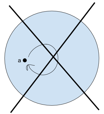
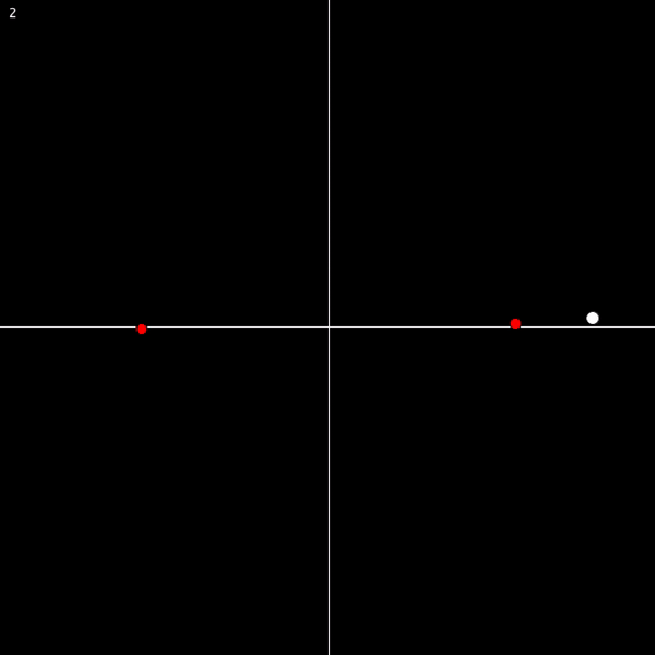
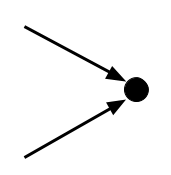
Visually, the first axiom tells us that this situation can’t happen:

Untitled document (1)

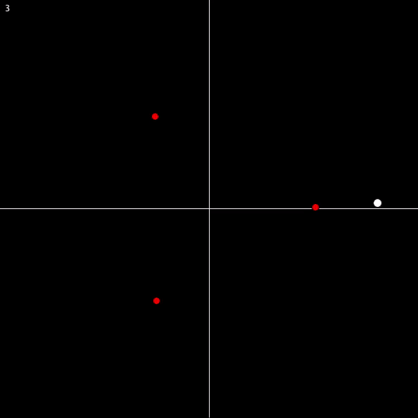
And the second axiom tells us that this situation can’t happen:

Now, we know that 0 is a number, because it’s a constant in our language.

Untitled document

By axiom 1, we know that S0 cannot be 0. So it’s something new.

Untitled document (3)

S0 cannot go to 0, because of axiom 1. And it can’t go to itself, as that would be a violation of axiom 2. So it has to go to something new:

Untitled document (4)

Now, where does SS0 get sent? Not to 0, for the same reason as before. And not to either S0 or SS0, because then we’d have a violation of axiom 2. So it must go to a new number. You can see where this is going.

Untitled document (5)

These two axioms really cleverly force us to admit an infinite chain of unique new numbers. So is that it? Have we uniquely pinned down the natural numbers?

It turns out that the answer is no. Consider the following model:

Untitled document (6)

This is perfectly consistent with our axioms! No number goes to 0 via the successor function, and no two different numbers have the same successor. But clearly this is not a model of the natural numbers. One quick and easy patch on this is just to add a new axiom, banning any numbers that are their own successor.

3. ∀x (Sx ≠ x)

Now, we’ve taken care of this problem, but it’s a symptom of a larger issue. Here’s a model that’s perfectly consistent with our new axioms:

Untitled document (7)

In the same vein as before, we can patch this with a new axiom, call it 3’:

3’. ∀x (SSx ≠ x)

But now we have the problem of three-loops, which require their own axiom to be ruled out (3’’. ∀x (SSSx ≠ x)). And in general, this approach will end up requiring us to have an infinite axiom schema, one axiom for each loop length that we need to ban.

However, even then we’re not done! Why? Well, once we’ve banned all loops, we run into the following problem:

Untitled document (8)

We can fix this by specifying that 0 is the only number that is not the successor of any number. Formally, this looks like:

∀x (∀y (Sy ≠ x) → x = 0)

Okay, so that takes care of other copies of the natural numbers. But we’re still not done! Take a look at the following model:

Untitled document (9)

This model violates none of our axioms, but is clearly not the natural numbers. We’re running into a lot of problems here, and our list of axioms is getting really long and unwieldy. Is there any simpler system of axioms that will uniquely pin down the natural numbers for us?

The amazing fact is that no, this is not possible. In fact, no matter how hard you try, you will never be able to rule out models of your axioms that contain “nonstandard numbers” in first-order logic.

We’ll prove this using a beautiful line of reasoning, which I think of as one of the simplest and most profound arguments I’ve encountered. There’s several subtle steps here, so read carefully:

Step 1

We’re going to start out by proving a hugely important theorem called the Compactness Theorem.

Suppose that a first order theory T has no model.
Then there is no consistent assignment of truth values to all WFFs.
So you can prove a contradiction from T. (follows from completeness)
All proofs must be finite, so if you can prove a contradiction from T, you can do it in a finite number of steps.
If the proof of contradiction takes a finite number of steps, then it uses only a finite number of T’s axioms.
So there is a proof of contradiction from a finite subset of T’s axioms.
So there’s a finite subset of T’s axioms that has no model. (follows from soundness)
So if T has no model, then there’s a finite subset of T’s axioms that has no model.

The Compactness Theorem as it’s usually stated is the contrapositive of this: If all finite subsets of T’s axioms have a model, then T has a model. If you stop to think about this for a minute, it should seem pretty surprising to you. (It’s trivial for the case that T contains a finite number of axioms, of course, but not if T has an infinity of axioms.)

Also notice that our proof of the theorem barely relied on what we’ve said about the properties of first order logic at all! In fact, it turns out that there is a Compactness Theorem in any logic that is sound (syntactic entailment implies semantic entailment, or in other words: that which is provable is true in all models), complete (semantic entailment implies syntactic entailment, or: that which is true in all models is provable), and only allows finite proofs.

In other words, any logic in which the provable statements are exactly those statements that are true in all models, no more and no less, and in which infinite proofs are considered invalid, will have this peculiar property.

Step 2

Now, we use the Compactness Theorem to prove our desired result.

Suppose we have a first order theory T that has the natural numbers N as a model.
We create a new theory T’ by adding a constant symbol ω and adjoining an infinite axiom schema:
- ‘ω ≥ 0’
- ‘ω ≥ S0’
- ‘ω ≥ SS0’
- ‘ω ≥ SSS0’ (And so on…)
N is no longer a model of T’, because T’ says that there is a number that’s larger than every natural number, which is false in N.
But T’ still has a model, because of compactness:
- Any finite subset of the axioms of T’ has a finite number of statements that look like ‘ω > x’. But this is consistent with ω being a natural number! (because for any set of natural numbers you can find a larger natural number)
- So N is a model of any finite subset of the axioms of T’.
- So by compactness, T’ has a model. This model is nonstandard (because earlier we saw that it’s not N).
Furthermore, any model of T’ is a model of T, because T’ is just T + some constraints.
So since T’ has a nonstandard model, so does T.
Done!

The conclusion is the following: Any attempt to model N with a first order theory is also going to produce perverse nonstandard models in which there are numbers larger than any natural number.

Furthermore, this implies that no first order theory of arithmetic can prove that there is no number larger than every natural number. If we could, then we would be able to rule out nonstandard models. But we just saw that we can’t! And in fact, we can realize that ω, as a number, must have a successor, which can’t be itself, and which will also have a successor, and so on forever, so that we will actually end up with an infinity of infinitely-large numbers, none of which we have any power to deny the existence of.

But wait, it gets worse! Compactness followed from just three super elementary desirable features of our logic: soundness, completeness, and finite provability. So this tells us that our inability to uniquely pin down the natural numbers is not just a problem with first order logic, it’s basically a problem with any form of logic that does what we want it to do.

Want to talk about the natural numbers in a Hilbertian logical framework, where anything that’s true is provable and anything that’s provable is true? You simply cannot. Anything you say about them has to be consistent with an interpretation of your statements in which you’re talking about a universe with an infinity of infinitely large numbers.

Löwenheim-Skolem Theorem

Just in case your mind isn’t sufficiently blown by the Compactness Theorem and its implications, here’s a little bit more weirdness.

The Löwenheim-Skolem Theorem says the following: If a first-order theory has at least one model of any infinite cardinality, then it has at least one model of EVERY infinite cardinality.

Here’s an intuition for why this is true: Take any first order theory T. Construct a new theory T’ from it by adding κ many new constant symbols to its language, for any infinite cardinality κ of your choice. Add as axioms c ≠ c’, for any two distinct new constant symbols. The consistency of the resulting theory follows from the Compactness Theorem, and since we got T’ by adding constraints to T, any model of T’ must be a model of T as well. So T has models of any infinite cardinality!

The Löwenheim-Skolem Theorem tells us that any first order theory with the natural numbers as a model also has models the size of the real numbers, as well as models the size of the power set of the reals, and the power set of the power set of the reals, and so on forever. Not only can’t we pin down the natural numbers, we can’t even pin down their cardinality!

And in fact, we see from this that no first-order statement can express the property of “being a specific infinite cardinality.” If we could do this, then we could just add this statement to a theory as an axiom and rule out all but one infinite cardinality.

Here’s one more for you: The Löwenhiem-Skolem Theorem tells us that any attempt to talk about the real numbers in first order logic will inevitably have an interpretation that refers solely to a set that contains a countable infinity of objects. This implies that in first order logic, almost all real numbers cannot be referred to!

Similarly, a first order set theory must have countable models. But keep in mind that Cantor showed how we can prove the existence of uncountably infinite sets from the existence of countably infinite sets! (Namely, just take a set that’s countably large, and power-set it.) So apparently, any first order set theory has countable models that… talk about uncountable infinities of sets? This apparent contradiction is known as Skolem’s paradox, and resolving it leads us into a whole new set of strange results for how to understand the expressive limitations of first order logic in the context of set theory.

All that and more in a later post!

Introduction to Mathematical Logic (Part 1)

October 6, 2019April 16, 2026 ~ ~ 3 Comments

Mathematical logic is the study of the type of reasoning we perform when we do mathematics, and the attempt to formulate a general language as the setting in which all mathematics is done. In essence, it is an attempt to form a branch of mathematics, of which all other branches of mathematics will emerge as special cases.

You might sort of think that when speaking at this level of abstraction, there will nothing general and interesting to say. After all, we’re trying to prove statements not within a particular domain of mathematics, but theorems that are true across a wide swath of mathematics, potentially encompassing all of it.

The surprising and amazing thing is that this is not the case. It turns out that there are VERY general and VERY surprising things you can discover by looking at the logical language of mathematics, a host of results going by names like the Completeness Theorem, the Incompleteness Theorem, the Compactness Theorem, the Löwenheim-Skolem Theorem, and so on. These results inevitably have a great deal of import to our attitudes towards the foundations of mathematics, being that they generally establish limitations or demonstrate eccentricities in the types of things that we can say in the language of mathematics.

My goal in this post is to provide a soft introduction to the art of dealing in mathematics at this level of ultimate abstraction, and then to present some of the most strange things that we know to be true. I think that this is a subject that’s sorely missing this type of soft introduction, and hope I can convey some of the subject’s awesomeness!

— — —

To start out with, why think that there is any subject matter to be explored here? Different branches of mathematics sometimes appear to be studying completely different types of structures. I remember an anecdote from an old math professor of mine, who worked within one very narrow and precisely defined area of number theory, and who told me that when she goes to talks that step even slightly outside her area of specialty, the content of the lectures quickly incomprehensible to her. Why think that there is such a common language of mathematics, if specialists in mathematics can’t even understand each other when talking between fields?

The key thing to notice here is that although different fields of mathematics are certainly wildly different in many ways, there nevertheless remain certain fundamental features that are shared in all fields. Group theorists, geometrists, and number theorists will all accept the logical inference rule of modus ponens (if P is true and P implies Q, then Q is true), but none of them will accept its converse (if Q is true and P implies Q, then P is true). No matter what area of mathematics you study, you will accept that if P(x) is true for all x, then it is true for any particular x you choose. And so on. These similarities may seem obvious and trivial, but they HAVE to be obvious and trivial to be things that every mathematician agrees on. The goal, then, is to formalize a language that has these fundamental inference rules and concepts built in, and that has many special cases to account for the differences between domains of math, specified by some parameters that are freely chosen by any user of the system.

There are actually several distinct systems that attempt to accomplish this task. Generally speaking, there are three main branches, in order of increasing expressive power: propositional logic, first order (predicate) logic, and second order logic.

Reasoning In Zeroth Order

Let’s start with propositional logic, sometimes called “zeroth order logic.” Propositional logic is the framework developed to deal with the validity of the following types of arguments:

Argument 1

2+2=4.
If 2+2=4, then 1+3=4.
So 1+3=4.

Argument 2

The Riemann hypothesis is false and P = NP.
So P = NP.

Notice that it doesn’t matter if our premises are true or not. Logical validity doesn’t care about this, it just cares that the conclusions really do follow from the premises. This is a sign of the great generality at which we’re speaking. We’re perfectly fine with talking about a mathematical system in which the Riemann hypothesis is false, or in which 2+2 is not 4, just so long as we accept the logical implications of our assumptions.

Propositional logic can express the validity of these arguments by formalizing rules about valid uses of the concepts ‘and’, ‘if…then…’, ‘or’, and so on. It remains agnostic to the subject matter being discussed by not fully specifying the types of sentences that are allowed to be used in the language. Instead, any particular user of the language can choose their set of propositions that they want to speak about.

To flesh this out more, propositional logic fulfills the following three roles:

Defines an alphabet of symbols.
Specifies a set of rules for which strings are grammatical and which are not.
Details rules for how to infer new strings from existing strings.

In more detail:

The set of symbols in propositional logic are split into two categories: logical symbols and what I’ll call “fill-in-the-blank” symbols. The logical symbols are (, ), ∧, ∨, ¬, and →. The fill-in-the-blank symbols represent specific propositions, that are specified by any particular user of the logic.
Some strings are sensible and others not. For example, the string “P∧∧” will be considered to be nonsensical, while “P∧Q” will not. Some synonyms for sensible strings are well-formed formulas (WFFs), grammatical sentences, and truth-apt sentences. There is a nice way to inductively generate the set of all WFFs: Any proposition is a WFF, and for any two WFFs F and F’, the following are also WFFs: (F∧F’), (F∨F’), ¬F, (F→F’).
These include rules like modus ponens (from P and P→Q, derive Q), conjunction elimination (from P∧Q, derive P), double negation elimination (from ¬¬P, derive P), and several more. They are mechanical rules that tell you how to start with one set of strings and generate new ones in a logically valid way, such that if the starting strings are true than the derived ones must also be true. There are several different but equivalent formulations of the rules of inference in propositional logic.

A propositional language fills in the blanks in the logic. Say that I want to talk about two sentences using propositional logic: “The alarm is going off”, “A robber has broken in.” For conciseness, we’ll abbreviate these two propositions as A for alarm and R for robber. All I’ll do to specify my language is to say “I have two propositions: {A, R}”

The next step is to fill in some of the details about the relationships between the propositions in my language. This is done by supplementing the language with a set of axioms, and we call the resulting constrained structure a propositional theory. For instance, in my example above we might add the following axioms:

A→R
A∨R

In plain English, these axioms tell us that (1) if the alarm is going off, then a robber has broken in, and (2) an alarm is going off or a robber has broken in.

Finally, we talk about the models of our theory. Notice that up until now, we haven’t talked at all about whether any statements are true or false, just about syntactic properties like “The string P∨¬ is not grammatical” and about what strings follow from each other. Now we interpret our theory by seeing what possible assignments of truth values to the WFFs in our language are consistent with our axioms and logical inference rules. In our above example, there are exactly two interpretations:

Model 1: A is true, R is true
Model 2: A is false, R is true

These models can be thought of as the possible worlds that are consistent with our axioms. In one of them, the alarm has gone off and a robber has broken in, and in the other, the alarm hasn’t gone off and the robber has broken in.

Notice that R turns out true in both models. When a formula F is true in all models of a theory, we say that the theory semantically entails F, and write this as T ⊨ F. When a formula can be proven from the axioms of the theory using the rules of inference given by the logic, then we say that the theory syntactically entails F, and write this as T ⊢ F.

This distinction between syntax and semantics is really important, and will come back to us in later discussion of several important theorems (notably the completeness and incompleteness theorems). To give a sneak peek: above we found that R was semantically entailed by our theory. If you’re a little familiar with propositional logic, you might have also realized that R can be proven from the axioms. In general, syntactic truths will always be semantic truths (if you can prove something, then it must be true in all models, or else the models would be inconsistent. But a model is by definition a consistent assignment of truth values to all WFFs). But a natural question is: are all semantic consequences of a theory also syntactic consequences? That is, are all universal truths of the theory (things that are true in every model of the theory) provable from the theory?

Summary of mathematical logic meeting

If the answer is yes, then we say that our logic is complete. And it turns out that the answer is yes, for propositional logic. Whether more complex logics are complete turns out to be a more interesting question. More on this later.

This four-step process I just laid out (logic to language to theory to model) is a general pattern we’ll see over and over again. In general, we have the following division of labor between the four concepts:

Logic: The logic tells us the symbols we may use (including some fill-in-the-blank categories of symbols), the rules of grammar, and a set of inference rules for deriving new strings from an existing set.
Language: The language fills in the blanks in our logic, fully specifying the set of symbols we will be using.
Theory: The theory adds axioms to the language.
Model: A model is an assignment of truth values to all WFFs in the language, consistent with the axioms and the inference rules of our logic.

It’s about time that we apply this four-step division to a more powerful logic. Propositional logic is pretty weak. Not much interesting math can be done in a purely propositional language, and it’s wildly insufficient to capture our notion of logically valid reasoning. Consider, for example, the following argument:

Socrates is a man.
All men are mortal.
So, Socrates is mortal.

This is definitely a valid argument. No rational agent could agree that 1 and 2 are true, and yet deny the truth of 3. But can we represent the validity of this argument in propositional logic? No!

Consider that the three sentences “Socrates is a man”, “All men are mortal”, and “Socrates is mortal” are distinct propositions, and the relationships between them are too subtle for propositional logic to capture. Propositional logic can’t see that the first proposition is asserting the membership of Socrates to a general class of things (“men”), and that the second proposition is then making a statement about a universal property of things in this class. It just sees two distinct propositions. To propositional logic, this argument just looks like

P
Q
Therefore, R

But this is not logically valid! We could make it valid by adding as a premise the sentence (P∧Q)→R, which corresponds to the English sentence “If Socrates is a man and all men are mortal, then Socrates is mortal.” But this should be seen as a tautology, something that is provable in any first order theory that contains the propositions P Q and R, not a required additional assumption. Worse, if somebody came along and stated the proposition A = “Aristotle is a man”, then we would need a whole ‘nother assumption to assert that Aristotle is also mortal! And in general, for any individual instance of this argument, we’d need an independent explanation for its validity. This is not parsimonious, and indicative that propositional logic is missing something big.

Missing what? To understand why this argument is valid, you must be able to reason about objects, properties, and quantification. This is why we must move on to an enormously more powerful and interesting logic: first order logic.

Reasoning In First Order

First order logic is a logic, so it must fill the same three roles as we saw propositional logic did above. Namely, it must define the alphabet, the grammar, and the inference rules.

Symbols
Logical: ∧ ∨ ¬ → ( ) ∀ ∃ =
Variables: x y z w …
Constants: ______
Predicates: ______
Functions: ______

That’s right, in first order we have three distinct categories of fill-in-the-blank symbols. Intuitively, constants will be names that refer to objects, predicates will be functions from objects to truth values, and functions will take objects to objects. To take an everyday example, if the objects in consideration are people, then we might take ‘a’ to be a constant referring to a person named Alex, ’T’ to be a predicate representing ‘is tall’, and ‘f’ to be a function representing “the father of”. So T(a) is either true or false, while f(a) doesn’t have a truth value (it just refers to another object). But T(f(a)) does have a truth value, because it represents the sentence “Alex’s father is tall.”

Next, we define well-formed formulas. This process is more complicated than it was for propositional logic, because we have more types of things than we did before, but it’s not too bad. We start by defining a “term”. The set of terms is inductively generated by the following scheme: All constants and variables are terms, and any function of terms is itself a term. Intuitively, the set of terms is the set of objects that our language is able to “point at”.

With the concept of terms in hand, we can define WFFs through a similar inductive scheme: Any predicate of terms is a WFF. And for any WFFs F and F’, (F∧F’), (F∨F’), (¬F), (F→F’), ∀x F, ∃x F are all WFFs. The details of this construction are not actually that important, I just think it’s nice how you can generate all valid first order formulas from fairly simple rules.

Good! We have an alphabet, a grammar, and now all we need from our logic is a set of inference rules. It turns out that this set is just going to be the inference rules from propositional logic, plus some new ones:

Quantifier elimination: From ∀x P(x) derive P(t) (for any term t and predicate P)
Quantifier introduction: From P(t) derive ∃x P(x) (for any term t and predicate P)

That’s it, we’ve defined first order logic! Now let’s talk about a first order language. Just like before, the language is just obtained by filling in the blanks left open by our logic. So for instance, we might choose the following language:

Constants: a
Functions: f
Predicates: none

In specifying our function, we have to say exactly what type of function it is. Functions can take as inputs a single object (“the father of”) or multiple objects (“the nearest common ancestor of”), and this will make a difference to how they are treated. So for simplicity, let’s say that our function f just takes in a single object.

A first order theory will simply be a language equipped with some set of axioms. Using our language above, we might have as axioms:

∀x (f(x) ≠ x)
∀x (f(x) ≠ a)

In plain English, we’re saying that f never takes any object to itself or to a.

And lastly, we get to the models of a first order theory. There’s an interesting difference between models here and models in propositional logic, which is that to specify a first order model, you need to first decide on the size of your set of objects (the size of the ‘universe’, as it’s usually called), and then find a consistent assignment of truth values to all propositions about objects in this universe.

So, for instance, we can start searching for models of our theory above by starting with models with one object, then two objects, then three, and so on. We’ll draw little diagrams below in which points represent objects, and the arrow represents the action of the function f on an object.

No 1-element universe.
No 2-element universe.
3-element universe
4 element universes
And so on…

It’s a fun little exercise to go through these cases and see if you can figure out why there are no models of size 1 or 2, or why the one above is the only model of size 3. Notice, by the way, that in the last two images, we have an object for which there is no explicit term! We can’t get there just using our constant and our functions. Of course, in this case we can still be clever with our quantifiers to talk about the Nameless One indirectly (for instance, in both of these models we can refer to the object that is not equal to a, f(a), or f(f(a))) But in general, the set of all things in the universe is not going to be the same as the set of things in the universe that we can name.

Here’s a puzzle for you: Can you make a first order sentence that says “I have exactly four objects”? That is, can you craft a sentence that, if added as an axiom to our theory, will rule out all models besides the ones that have exactly four elements?

(…)

(Think about it for a moment before moving on…)

(…)

Here’s how to do it for a universe with two objects (as well as a few other statements of interest). The case of four objects follows pretty quickly from this.

“I have at most two objects” = ∃x∃y∀z (z=x ∨ z=y)
“I have exactly two objects” = ∃x∃y (x≠y ∧ ∀z(z=x ∨ z=y))
“I have at least two objects” = ∃x∃y (x≠y)

Another puzzle: How would you say “I have an infinity of objects”, ruling out all finite models?

(…)

(Think about it for a moment before moving on…)

(…)

This one is trickier. One way to do it is to introduce an infinite axiom schema: “I have at least n objects” for each n.

This brings up an interesting point: theories with infinite axioms are perfectly permissible for us. This is a choice that we make that we could perfectly well deny, and end up with a different and weaker system of logic. How about infinitely long sentences? Are those allowed? No, not in any of the logics we’re talking about here. A logic in which infinite sentences are allowed is called an infinitary logic, and I don’t know too much about such systems (besides that propositional, first, and second order logics are not infinitary).

Okay… so how about infinitely long derivations? Are those allowed? No, we won’t allow those either. This one is more easy to justify, because if infinite derivations were allowed, then we could prove any statement P simply by the following argument “P, because P, because P, because P, because …”. Each step logically follows from the previous, and in any finite system we’d eventually bottom out and realize that the proof has no basis, but in a naive infinite-proof system, we couldn’t see this.

Alright, one last puzzle. How would you form the sentence “I have a finite number of objects”? I.e., suppose you want to rule out all infinite models but keep the finite ones. How can you do it?

(…)

(Think about it for a moment before moving on…)

(…)

This one is especially tricky, because it turns out to be impossible! (Sorry about that.) You can prove, and we will prove in a little bit, that no first order axiom (or even infinite axiom schema) is in general capable of restricting us to finite models. We have run up against our first interesting expressive limitation of first-order logic!

Okay, let’s now revisit the question of completeness that I brought up earlier. Remember, a logic is complete if for any theory in that logic, the theory’s semantic implications are the same as its syntactic implications (all necessary truths are provable). Do you think that first order logic is complete?

The answer: Yes! Kurt Gödel proved that it is in his 1929 doctoral dissertation. Anything that is true in all models of a first order theory, can be proven from the axioms of that theory (and vice versa). This is a really nice feature to have in a logic. It’s exactly the type of thing that David Hilbert was hoping would be true of mathematics in general. (“We must know. We will know!”) But this hope was dashed by the same Kurt Gödel as above, in his infamous incompleteness theorems.

There will be a lot more to say about that in the future, but I’ll stop this post for now. Next time, we’ll harness the power of first order logic to create a first order model of number theory! This will give us a chance to apply some powerful results in mathematical logic, and to discover surprising truths about the logic’s limitations.

Thinking in first order: Are the natural numbers countable?

September 30, 2019September 30, 2019 ~ ~ 1 Comment

Here’s a weird fact about first-order logic: there is no first-order theory that has as a model the natural numbers and only the natural numbers. Any first-order theory talking about N can only say things that are also consistent with weird other systems that include uncountable infinities of nonstandard numbers. Here’s the proof:

Take first order Peano arithmetic (PA). We know that the natural numbers N are a model of PA, because all the axioms are true of PA. Now add a constant c to your language, and adjoin an infinite axiom schema: ‘c > 0’, ‘c > S0’, ‘c > SS0’, and so on. Call this new theory PA(c).

The natural numbers are clearly no longer a model of PA(c), because PA(c) says that there’s a number that’s larger than all natural numbers, which is false in N. But we can prove that PA(c) still has a model! We prove this using the Compactness Theorem, which tells us that a theory has a model if every finite subset of its axioms has a model. Consider any finite subset of the axioms of PA(c). For any such subset, there are only finitely many statements that look like c > X. So there are only finitely many numbers that c is larger than. But then this is always going to be satisfied by N! For any collection of natural numbers, you can always find a natural number larger than all of then. So N is a model of every finite subset of the axioms of PA(c). But then, by compactness, since every finite subset of the axioms of PA(c) has a model, PA(c) has a model!

Final step in the proof: PA(c) has a model, and this model is definitely not the natural numbers. Call it a nonstandard model. But now note that PA(c) was obtained from PA just by adding axioms. Adding axioms never increases the number of models, it only narrows them down. So if the nonstandard model is a model of PA(c), then it also must be a model of PA! And there it is, we’ve proved that first order Peano arithmetic has more models than the natural numbers.

Notice, also, that it didn’t matter that we started with first order Peano arithmetic. We could have started with any first order theory that has N as a model, added the constant c, and adjoined on the infinite axiom schema corresponding to c being larger than all natural numbers! So what we’ve actually proven is that no first order theory can “pin down” the natural numbers. Any first order theory that has N as a model, also has weird extra models that allow numbers greater than all natural numbers. Furthermore, you can then run the exact same type of proof again, adjoining a new constant that’s larger than all natural numbers and also larger than c, and by compactness show that it has a model, so that you’ve now found that any first order theory that has N as a model also has a model that has the natural numbers, plus a number larger than all natural numbers, plus a number that’s larger than even that. And you can do this an uncountable infinity of times, and end up proving that if your favored theory has N as a model, then it also has a model whose size is an uncountable infinity. And in fact, any first order theory that has N as a model, also has models of every infinite cardinality.

This is super wild, and really important. Why does it matter that we can’t pin down the natural numbers using any first order theory? Well, think about the set of statements that are true of N, but false of these nonstandard models. These include “there is no number larger than all natural numbers” and “There are a countable infinity of natural numbers”. These statements are not true in all models of any first order theory of N. And if they’re false in some models, then they can’t be proven from the axioms of the theory! (If the theory could prove a statement that was false in one of its models, then the model wouldn’t have been a model of the theory in the first place; models are consistent assignments of truth values to the sentences of the theory.)

In other words, no first order theory of the natural numbers can prove that the natural numbers are countable, or that no number is greater than all natural numbers. If you were a being that could only think in first-order sentences, then you would be unable to conclude these basic facts. To say these things, you need to go up a level to second-order logic, and quantify over properties in addition to objects. Even weirder, if you could only think in first-order logic, you wouldn’t even be able to talk about the natural numbers. No matter how hard you tried to say what you meant by the natural numbers, you would always fail to pin down just the natural numbers. There’d always be room for ambiguity, and everything you said and thought could be equally well interpreted as being about some bizarre non-standard model.

Extending this one step further, there’s a theorem in mathematical logic called the Löwenheim-Skolem Theorem. This theorem generalizes what we showed above about the natural numbers: any first order theory that has a model with countably infinite size, also has models with size every cardinality of infinity. So no first order theory can prove a statement that is true of countably infinite sets but false of uncountably infinite sets. And actually, the theorem is even stronger than that: any theory that has a model of any infinite cardinality, must also have models of all infinite cardinalities! So, for instance, any first order theory of the real numbers has a model that is the size of N! To first order logic, there is no expressible difference between the different infinite cardinalities. The statements “this size of this set is countable infinity” or “the size of this set is uncountable infinity” can’t be said in any first-order language, as doing so would cut out the models of other cardinalities, which the Löwenheim-Skolem Theorem tells us can’t happen.

A Talmudic Probability Puzzle

September 2, 2019 ~ ~ 2 Comments

Today we’ll take a little break from the more intense abstract math stuff I’ve been doing, and do a quick dive into a fun probabilistic puzzle I found on the internet.

Background for the puzzle: In Ancient Israel, there was a court of 23 wise men that tried important cases, known as the Sanhedrin. If you were being tried for a crime by the Sanhedrin and a majority of them found you guilty, you were convicted. But there was an interesting twist on this! According to the Talmud (Tractate Sanhedrin: Folio 17a), if the Sanhedrin unanimously found you guilty, you were to be acquitted.

If the Sanhedrin unanimously find [the accused] guilty, he is acquitted. Why? — Because we have learned by tradition that sentence must be postponed till the morrow in hope of finding new points in favour of the defence. But this cannot be anticipated in this case.

Putting aside the dubious logic of this rule, it gives rise to an interesting probability puzzle with a counterintuitive answer. Imagine that an accused murderer has been brought before the Sanhedrin, and that the evidence is strong enough that no judge has any doubt in their mind about his guilt. Each judge obviously wants for the murderer to be convicted, and would ordinarily vote to convict. But under this Talmudic rule, they need to be worried about the prospect of them all voting guilty and therefore letting him off scot-free!

So: If a probability p can be chosen such that each and every judge votes to convict with probability p, and to acquit with probability 1 – p, which p will give them the highest probability of ultimately convicting the guilty man?

Furthermore, imagine that the number of judges is not 23, but some arbitrarily high number. As the number of judges goes to infinity, what does p converge to?

I want you to think about this for a minute and test your intuitions before moving on.

(…)

So, it turns out that the optimal p for 23 judges is actually ≈ 75.3%. And as the number of judges goes to infinity? The optimal value of p converges to…

80%!

This was a big shock to me. I think the natural first thought is that when you have thousands and thousands of judges, you only need a minuscule chance for any one judge to vote ‘acquit’ in order to ensure a majority and prevent him from getting off free. So I initially guessed that p would be something like 99%, and would converge to 100% in the limit of infinite judges.

But this is wrong! And of the small sample of mathematically gifted friends I asked this question to, they mostly guessed the same as me.

There’s clearly a balance going on between the risk of a minority voting to convict and the risk of a unanimous vote to convict. For small p, the first of these is ~1 and the second is ~0, and for p ~ 1, the first is ~0 and the second ~1. It seems that we are naturally underemphasizing the danger of a minority vote to convict, and overemphasizing the danger of the unanimous vote.

Here are some plots of the various relevant values, for different numbers of judges:

10 Judges 23 Judges 100 Judges 150 Judges

One thing to notice is that as the number of judges gets larger, the graph’s peak becomes more and more of a plateau. And in the limit of infinite judges, you can show that the graph is actually just a simple step function: Pr(conviction) = 0 if p < .5, and 1 if p > .5. This means that while yes, technically, 80% is the optimal value, you can do pretty much equally well by choosing any value of p greater than 50%.

My challenge to you is to come up with some justification for the value 80%. Good luck!

Galois’ Unsolvable Polynomials

September 1, 2019April 16, 2026 ~ ~ Leave a comment

Galois’ process for finding out if a polynomial is solvable by radicals (i.e., if you can write its roots using a finite number of rational numbers and the symbols +, -, ×, /, and √) is actually surprisingly simple to describe. Here’s a quick 4-step summary of the process:

Take a polynomial p(x).
Define E to be the smallest field that contains all rational numbers, as well as all the roots of p(x). This field is called the splitting field of p(x).
Define Gal(E/Q) to be the set of all isomorphisms from E to itself that hold fixed all rational numbers. This set is a group, and is called the Galois group of p(x).
p(x) is solvable by radicals if and only if Gal(E/Q) is a solvable group.

The proof of (4) is pretty complicated (much more involved than the proof I gave in the last post). Galois’ method is also a little weaker in that it only allows you to conclude unsolvability using the symbols +, -, ×, /, and √, whereas the last post also concluded unsolvability with √ as well as any univalent function (exp, log, sin, or whatever). However, it does allow you to not just generally state that some order-five polynomials are not solvable by radicals, but to determine for any given polynomial whether it is solvable. The process also gives you a good deal of insight into the nature of the roots of the polynomial you’re studying.

Now, the crucial step in this 4-step process is (4), which equates solvable polynomials with solvable groups. There are a few different but equivalent definitions of solvable groups:

Composition Series Definition

A composition series of G is a series of subgroups of G, such that each subgroup is a maximal normal subgroup of the previous subgroup (maximal means that no normal subgroup contains it besides G itself).
- {1} = G₀ ◃ G₁ ◃ … ◃ G_n = G.
G is solvable if and only if the factors of its composition series are all cyclic of prime order (i.e. if for all k, G_k+1/G_k ≅ ℤ_p for prime p).

Derived Series Definition

The derived series of G is the series of subgroups where each subgroup is the commutator subgroup of the previous subgroup.
- … ◃ [[G,G], [G,G]]◃ [G, G] ◃ G.
G is solvable if and only if this series eventually reaches the trivial group.

Subnormal Series Definition

A subnormal series of G is a series of subgroups of G where each subgroup is a normal subgroup of the previous subgroup, and which terminates in the trivial group.
- {1} = G₀ ◃ G₁ ◃ … ◃ G_n = G.
G is solvable if and only if all the factors of a subnormal series of G are abelian.

Solvability is an interesting group-theoretic property aside from its application in analyzing polynomial roots. Here are some things we know about solvable groups, in order of generally decreasing power:

Every group of odd order is solvable.
Every abelian group is solvable.
Every group of prime power order is solvable. (i.e. if |G| = pⁿ for prime p and any n)
Every group of product of prime powers order is solvable. (i.e. if |G| = pⁿq^m for primes p, q and any n, m)
Every group whose Sylow subgroups are cyclic is solvable.
No finite non-abelian simple groups are solvable.
If H and G/H are solvable, then G is solvable.
S_n is not solvable for all n ≥ 5.
Dihedral groups are all solvable.

A fun exercise is to see how many of these you can prove. (Some are much easier than others, and in fact the first one took 255 pages to prove!)

It turns out that most groups are solvable. In fact, the smallest non-solvable group has 60 elements (A₅). Here’s the first few numbers in the sequence of sizes of non-solvable groups:

60, 120, 168, 180, 240, 300, 336, 360, 420, 480, 504, 540, 600, 660, 672, 720, 780, 840, 900, 960, …

Determining the elements of Gal(E/ℚ)

Practically, the hardest part of the above 4-step process is determining what the Galois group is for a given polynomial. Usually one knows very little about the roots of the polynomial in question, and therefore also knows little about its splitting field. So how to determine the Galois group (the set of automorphisms of the splitting field that fix ℚ) without even knowing what the splitting field is? Well, it turns out that there are some really useful general tricks.

For one: Sometimes you can look closely at the polynomial and discover some simple algebraic relations that must hold among the roots. For instance, say p(x) = x⁴ + 2x² – 1. Since there are only even powers of x in p(x), for any root r of p(x), -r must also be a root. This means that roots of p(x) can be written {A, -A, B, -B} for some reals A and B. And by the properties of homomorphisms, whichever root X that A is mapped to by a member of the Galois group, -A must also map to -X. Another way to say this is that the Galois group of any even polynomial is not the full group of permutations of the roots S_n (as the evenness imposes the above restriction on the allowed automorphisms).

A superb trick related to this is to look at the modular algebraic relations between roots. In general, you can take a complicated irreducible polynomial, and break it into smaller irreducible factors modulo a prime p. Dedekind’s theorem tells us that if there are no repeated factors, then the Galois group contains permutations of the roots with cycle type corresponding to the degrees of the factors.

Example 1

Let p(x) = x² – 1.
The splitting field E of p(x) is clearly ℚ(√2) = {a + b√2 for all a, b in ℚ}.
Gal(E/ℚ) = the set of automorphisms on E that hold fixed all rationals.
If f is in Gal(E/ℚ), then f(√2)² = f(√2 × √2) = f(2) = 2. So f(√2) = ±√2. So there are two automorphisms in Gal(E/ℚ): f(a + b√2) = a + b√2 and f(a + b√2) = a – b√2.
So Gal(E/ℚ) ≅ ℤ₂
Since ℤ₂ is solvable, so p(x) is solvable (as was obvious from the outset).

Example 2

Let p(x) = x⁵ + x⁴ + x + 3. Then we can write:

p(x) = (x + 1)(x² + x + 1)(x³ + x + 1) mod 2
p(x) = x(x + 2)(x⁴ + x³ + 2x² + 2x + 2) mod 3
p(x) = (x + 3)² (x⁴ + 4x³ + 3x² + x + 2) mod 5
p(x) = (x² + 5x + 2)(x⁴ + 2x³ + 3x² + 2x + 5) mod 7
p(x) = (x + 6)(x⁵ + 5x⁴ + 4x³ + 9x² + x + 6) mod 11
p(x) = (x² + 8x + 1)(x² + 9x + 10)(x² + 9x + 12) mod 13

From this and Dedekind’s theorem we can conclude:

Gal(E/ℚ) contains a permutation of cycle type (1,2,3)
Gal(E/ℚ) contains a permutation of cycle type (1,1,4): a 4-cycle
Repeated factor of x+3, so we don’t learn anything
Gal(E/ℚ) contains a permutation of cycle type (2,4)
Gal(E/ℚ) contains a permutation of cycle type (1,5): a 5-cycle
Gal(E/ℚ) contains a permutation of cycle type (2,2,2)

This automatically gives us a lot of insight into Gal(E/ℚ)! We have permutations of the form:

(a b)(c d e)
(a b c d)
N/A
(a b)(c d e f)
(a b c d e)
(a b)(c d)(e f)

We can go further and show that the only group of automorphisms that contains all of these types of elements is S₅. (Every symmetric group can generated by a transposition and a cycle. We have a cycle by #5, and we can get a cycle by cubing #1.) And since S₅ is not solvable (its commutator subgroup is A₅, whose commutator subgroup is itself, and thus the derived series never terminates), the polynomial x⁵ + x⁴ + x + 3 is not solvable by radicals.

One final note: There is a fantastic computational algebra system designed to solve problems in high-level mathematics known as Magma. There’s an online Magma calculator here which is free to use. To use it to find the Galois group of the above polynomial (for example), you type:

P<x>:=PolynomialRing(Rationals());
GaloisGroup(x^5+x^4+x+3);

The Inverse Galois Problem

Now we get to the most tantalizing part!

Instead of starting with a polynomial p(x) and finding its Galois group, one could equally well start with a group G and ask whether G is the Galois group of any polynomial with rational coefficients! If so, we say that G is realizable, and is realized by p(x).

It turns out that whether or not every finite group is realizable turns out to be one of the big unsolved questions in mathematics. We’d like to prove that you can find a polynomial with coefficients from ℚ with Galois group G, for every finite group G, but in general it’s not known if this is possible! This paper lists all the non-abelian simple groups of cardinality 100 million that are currently not known to be realizable.

We do know the answer for some general categories of groups. Here are some things that are known, in order of decreasing strength.

All solvable groups are realizable.
All finite abelian groups are realizable.
All the symmetric and alternating groups are realizable.
All cyclic groups are realizable (special case of finite abelian groups being realizable)
25 of the 26 sporadic groups are known to be realizable (the missing sporadic group is the Mathieu group M₂₃, whose realizability remains an open question).
- Amazingly, this implies the existence of a polynomial with rational coefficients whose Galois group is the Monster group!

x^5 – x – 1

August 27, 2019July 31, 2020 ~ ~ 2 Comments

One of the strange and wonderful facts of mathematics is the general unsolvability of quintic polynomials. If you haven’t heard about this, prepare to have your mind pleasantly blown. Most people memorize the quadratic equation, the general expression for the roots of any quadratic polynomial, in high school:

Screen Shot 2019-08-27 at 11.14.31 AM.png

And even though very few people learn it in school, it turns out that we know a general solution to any cubic polynomial as well. It’s a little cumbersome to write, but just like the quadratic equation, it expresses the zeroes of any cubic polynomial as a function of its coefficients.

ax³ + bx² + cx + d = 0
x = (some big complicated function of a, b, c, and d)

And in fact we have a general solution for any quartic polynomial as well, even more cumbersome.

ax⁴ + bx³ + cx² + dx + e = 0
x = (some even bigger and more complicated function of a, b, c, d, and e)

Mathematicians struggled for a long time to find a general solution for the roots of quintic polynomials (ax⁵ + bx⁴ + cx³ + dx² + ex + f = 0). Eventually, some mathematicians began to suspect that no such general solution existed. And then in the first few decades of the 1800s, a few mathematicians put out proofs to that effect. The most complete of these proofs was provided by Évariste Galois before he died in a duel at the age of 20 (we really need a big Hollywood movie about Galois’ life).

I recently found a fantastic 15-minute video sketching the proof of the unsolvability of the quintic. The approach taken in this proof is different from any of the original proofs, and it’s much simpler in a bunch of ways.

Here’s the video:

And briefly, here’s a summary of the proof:

The roots of any quintic polynomial obviously depend on the coefficients of the polynomial.
If you imagine taking a particular quintic polynomial (ax⁵ + bx⁴ + cx³ + dx² + ex + f), and making small continuous changes in the coefficients (a, b, c, d, e, f), then the set of zeroes of this polynomial should make similar continuous changes.
If you move each coefficient in a loop in the complex plane, ending at the same value it started at, then you should end up with the same set of zeroes as you started with (the same set, by the way, which doesn’t guarantee that each solution ends at the same place it started).
However, moving each coefficient in a loop in the complex plane sometimes ends up with the solutions switching places. (Illustration below)
For any “ordinary” function of the coefficients (a function that can be written using a finite number of rational numbers and the symbols +, -, ×, /, exp(), log(), √, and so on), you can find loops that don’t cause the solutions to switch places.
But for some quintic polynomials, you can always finds one of these loops that does cause the roots to switch places.
So there are quintic polynomials whose roots cannot be written as any ordinary function of the coefficients (since you can find a loop that permutes the solutions of the quintic but don’t permute the values of any ordinary function).

There are obviously holes in this proof that need to be filled. (1) through (3) should be pretty self-explanatory. And (4) can be illustrated by thinking about functions that involve square roots… on the complex plane, taking a square root of an expression means halving the angle to the expression. So rotating an expression around the complex plane by 2π only ends up rotating its square root by π (and thus bringing it to a different point). Observe:

Square Roots of 2 — Red dots are the square roots of the white dot, which starts and ends at 2.

And in general, a function involving an nth root of some ordinary expression will take n rotations around the complex plane to return each solution to its starting point. Take a look for n = 3:

Cube Roots of 2 — Red dots are the cube roots of the white dot, which starts and ends at 2.

For (5), you can prove this by using commutator loops (which are formed from two smaller loops L₁ and L₂ by putting them together as follows: L₁ L₂ L₁^-1 L₂^-1). Ultimately, this works for expressions with roots in them because solutions switch places exactly when you circle the origin of the complex plane, and commutators circle the origin a net zero times. For expressions with one nested root, you actually need to use commutators of commutators (first to return the inner root to its starting value, and then to return the outer root to its starting value). And with two nested roots, you use commutators of commutators of commutators. And so on. In this way, you can construct a loop in the complex plane for any expression you construct from roots and ordinary functions that will bring all values back to their starting points.

And finally, (6) is a result of the structure of the permutation group on five elements (S₅). If you look at all commutators of permutations of five elements, you are looking at the commutator subgroup of S₅, which is A₅ (the set of even permutations of five elements). And the commutator subgroup of A₅ is just A₅ itself. This means that you can find always find some commutator, or some commutator of commutators, or some commutator of commutators of commutators, (and so on) that is not equal to the identity permutation! (After all, if all commutators of commutators of commutators ended up just being the identity permutation, then the group of commutators of commutators of commutators would just be the trivial group {e}. But we already know that the group of commutators of commutators of commutators is just the commutator subgroup of the commutator subgroup of the commutator subgroup of S₅. I.e. the commutator subgroup of A₅, which is A₅.

And that’s the proof! You can see the whole thing sketched out in much more detail here.

Now, notice that the conclusion was that there are quintic polynomials whose roots cannot be written as any ordinary function of the coefficients. Not that all quintic polynomials’ roots can’t be written as such. Obviously, there are some quintics whose solutions can be written easily. For example…

x⁵ – 1 = 0
Solutions: x = e^2πik/5 for k = 0, 1, 2, 3, 4

But there also exist many quintic polynomials whose roots just have no way of being finitely expressed through ordinary functions! An example of this is the real root of x⁵ – x – 1.

x⁵ – x – 1 = 0
at x ≈ 1.167304…

Screen Shot 2019-08-27 at 11.24.41 AM — Plot of x⁵ – x – 1

There is no way to write this number using a finite number of the symbols +, -, ×, /, exp(), log(), √, sin(), cos(), and rational numbers. And this is the case even though this number is an algebraic number! I don’t know if there’s a name for this category of “algebraic numbers that cannot be explicitly expressed using ordinary functions” but there should be.

Of course, you can define a function into existence that just returns the solutions of the quintic (which is what the Bring radical allows one to do). And you can also write the solution with ordinary functions if you’re allowed to use an infinity of them. For example, you can use a repeated fifth root:

x⁵ – x – 1 = 0
x⁵ = x + 1
x = (1 + x)^1/5x = (1 + (1 + x)^1/5)^1/5x = (1 + (1 + (1 + x)^1/5)^1/5)^1/5x = (1 + (1 + (1 + (…))^1/5)^1/5)^1/5

But while an infinity of symbols suffices to express this 1.167304…, no finite number cuts it!

Group Theory: The Mathematics of Symmetry?

August 21, 2019August 22, 2019 ~ ~ Leave a comment

Often you’ll hear people describe group theory as being “the mathematics of symmetry.” If you’ve been exposed to a little bit of group theory, you might find this a little mystifying. While there are some subsets of group theory that explicitly pertain to symmetry (in particular, the dihedral groups, representing the symmetries of regular polygons), there are many more groups that seem to have nothing to do with symmetry (the rational numbers, for example, or the dicyclic groups). Much of group theory involves proving theorems about the structure of groups in abstract, and many of these theorems again seem to tell us little to nothing about symmetry (what does “for every prime p that divides the size of a group G, there is a subgroup of G with order p” mean as a statement about the nature of symmetry?). So what’s up? Why this identification between groups and symmetry?

Well, I think we can start with asking what we even mean by ‘symmetry’. The first thing I think of when I hear the word ‘symmetry’ is geometric symmetry – the rotations, translations, and reflections that hold fixed a given shape. This is indeed one big part of symmetry, but not all of it. Symmetry is huge in physics as well, and the meaning in this context is rarely geometric symmetry. Instead, ‘symmetry’ finds its deepest application in the notion of symmetries of nature, meaning transformations that hold fixed the form of the laws of nature. For instance, the behavior of physical systems would be identical if we were to uniformly “slide” the universe in one direction by some fixed amount. So the laws of nature must be invariant with respect to this type of uniform translation, and we say that uniform spatial translation is a symmetry of nature. But the behavior of physical systems would be affected if we, say, began uniformly accelerating all of space in some direction. So uniform acceleration is not a symmetry of nature, and the laws of nature will be sensitive to these types of transformations. In this context, symmetry is more or less synonymous with invariance.

What’s the similarity between these two senses of symmetry? Invariance really is the key. Geometric symmetries are transformations that hold fixed certain geometric properties; physical symmetries are transformations that hold fixed certain physical properties. Fundamentally, symmetries are transformations that hold fixed some quantity. When you choose strange abstract qualities, your symmetries can get pretty weird (like the invariance of magnetic fields with respect to addition of curl-less vector fields to the magnetic vector potential, one of the two gauge symmetries of Maxwell’s equations). But they are symmetries nonetheless!

Now, how does this expansive concept of symmetries relate to groups? Well, looking at the group axioms, it becomes fairly obvious that they do actually fit pretty well with the concept. Let’s think of the elements of a group as transformations one could perform upon a system, and the group operation as being ‘transformation composition’ for successive transformations. And finally, we think of the group as being a complete set of symmetries. Now we’ll look at what the group axioms say, one at a time.

Closure
For any two elements a, b in G, a•b is in G.
– Translation: If two transformations each individually hold fix some quantity, then doing the two transformations successively will also hold fixed the quantity.
Associativity
For any a, b, c in G, (a•b)•c = a•(b•c)
– Translation: The order in which transformations are applied to an object is all that determines the nature of the net transformation. The notion of parentheses doesn’t make sense in this context, there is only the left-to-right order of the application of transformations.
Identity
There is an element e in G such that for any a in G, a•e = e•a = a.
– Translation: Doing nothing at all holds fixed whatever quantity you choose.
Inverses
For any a in G, there is an element a’ in G such that a•a’ = e
– Translation: Any transformation that holds fixed some quantity will also hold fixed that quantity if done in reverse.

Put together, we see that it makes sense to think about a group as the complete set of reversible transformations that hold fixed a certain quantity. (To be clear, this indicates that any such set of symmetries can be treated as a group, not necessarily that any group can be regarded as a set of symmetries. However, this does turn out to be the case! And in fact, any group whatsoever can be considered as a set of geometric symmetries of some abstract object!)

“Complete” needs to be fleshed out a bit more. When talking about a set of transformations, we need to be picking from a well-defined starting set of ‘allowed transformations’. For example, sets of geometric symmetries of objects are usually drawn from the set of all isometries (transformations that keep all distances the same, i.e. rotations, reflections, and translations). Instead of this, we could also consider the allowed transformations to be restricted to the set of all rotations, in which case we’d just be looking at the set of all rotations that don’t change the object. But in general, we are not allowed to talk about the set of possible transformations as just being some subset of the set of all rotations. Why? Because we require that the set of allowed transformations be closed. If a certain rotation is in consideration as an allowed transformation of an object, then so must be twice that rotation, thrice it, and so on. And so must be the reverse of that rotation. Not all sets of rotations satisfy this constraint!

The general statement is that the set of allowed transformations from which we draw our set of symmetries must be closed. And if it is, then the resulting set of symmetries is well described as some group!

So there is a fairly simple sense in which group theory is the study of symmetries. There are the obvious geometric symmetries that I already mentioned (the dihedral groups). But now we can think further about what other familiar groups are actually symmetries of. (ℤ, +) is a group, so what are the integers symmetries of? There’s actually a few answers that work here. One is that ℤ is the set of translational symmetries of an infinite line of evenly spaced dots. Translating to the right corresponds to positive numbers, to the left is negatives, and no translation at all is 0. What about (ℤ_n, +)? It is the set of rotational symmetries of a circle with n dots placed evenly along its perimeter. I encourage you to try to think about other examples of groups (symmetric and alternating groups, ℚ, and so on), and how to think about them as symmetry groups.

This way of thinking about groups is more than just visually appealing, it actually helps clarify some otherwise opaque results in group theory. For example, why is the stabilizer of a group action always a subgroup? Well, the group action defines a set of allowed transformations, and the stabilizer of x is exactly the set of transformations that hold x fixed! So we have an invariant quantity x, and thus it is perfectly reasonable that the stabilizer should be a group.

Thinking of groups as sets of symmetries also allows us a nice physical interpretation of the idea of conjugacy classes, a hugely important tool in group theory. Remember, the conjugacy class of an element x in G is just the set of all conjugates of x; Cl(x) = {gxg^-1 for all g in G}. This ABA^-1 pattern might be familiar to you if you’ve studied a little bit of matrix representations of coordinate systems in physics. In this context, ABA^-1 just represents a coordinate transformation of B! First we apply some transformation A that changes our reference frame, then we apply B, and then we undo A to come back to the original reference frame. The result is basically that we get a transformation that are just like B, but in a different reference frame! So it makes perfect sense to think of the conjugacy class of an element x as just the set of all elements of the same “type” as x.

For a dihedral group, we get one conjugacy class for the identity, another for all rotations, and another for all flips. Why? Well every flip can be represented as any other flip in a rotated reference frame! And similarly, every rotation can be represented as any other rotation in a flipped reference frame. And of course, the do-nothing transformation will look the same in all reference frames, which is why the identity has its own conjugacy class. And for another example, you can see some great visualizations of the conjugacy class breakdown of the cube’s symmetry group here, under Examples at the top. In general, looking at conjugacy classes is a good way to get a sense of the natural breakdown of categories in your set of symmetries.

Now, the famous theorems about group structure (Lagrange, Cauchy, Sylow) all have intriguing interpretations as applied to symmetries. Why must it be that any object with a prime number of symmetries cannot have any non-trivial smaller complete sets of symmetries? And doesn’t it seem totally non-obvious that an object that has a complete set of symmetries whose size is divisible by 3, say, must also have a smaller complete set of symmetries (one drawn from a smaller closed set of allowed transformations) whose size is 3? But it’s true! Think about the symmetries of a regular triangle. There are six of them, and correspondingly there’s a closed set of symmetries of size 3, namely, the do-nothing transformation and the two rotations! And the same thing applies for any symmetry group of size 3N.

Furthermore, Sylow’s theorems give us really strong constraints on the number of subgroups of various sizes, none of which seem at all intuitive. Why must it be that if an object has 9N symmetries for some N that’s not divisible by 3, then N must be divisible by the number of smaller complete sets of symmetries?? Thinking about and trying to make intuitive sense of these connections is quite mind-boggling to me.

Symmetries of Platonic Solids

August 19, 2019August 19, 2019 ~ ~ Leave a comment

Definition: A polyhedron is regular if all its faces are the same regular polygon, and all angles are equal.

It turns out that there are only five Platonic solids (convex regular polyhedra).

Here’s a quick proof:

For a regular n-gon, the sum of its interior angles is (n – 2)π.
So the angle at any one of its corners must be (n – 2) π/n.
Now, suppose we have r faces (each a regular n-gon) meeting at every vertex.
Since the meeting point for each face is a corner with angle (n – 2)π/n, we have that the sum of the angles is r (n – 2) π/n.
And since the polyhedron is convex we must have r (n – 2) π/n < 2π.
This can be rewritten as (r – 2)(n – 2) < 4.
The only positive integers satisfying this are (n, r) = (3, 3), (4, 3), (3, 4), (5, 3), (3, 5).
These are our five Platonic solids!

(3,3): Tetrahedron

File:Tetrahedron.gif

Symmetry group: S₄

(4,3): Cube

File:Hexahedron.gif

Symmetry group: S₄ × ℤ₂

(3,4): Octahedron

File:Octahedron.gif

Symmetry group: S₄ × ℤ₂

(5,3): Dodecahedron

File:Dodecahedron.gif

Symmetry group: A₅ × ℤ₂

(3,5): Icosahedron

File:Icosahedron.gif

Symmetry group: A₅ × ℤ₂

— — —

Here’s one more thing to notice; when looking at small dihedral groups, we saw that Dih₃ (the symmetry group for a regular triangle) was isomorphic to S₃ (the set of permutations of three items). We also saw that this isomorphism did not hold for higher order dihedral groups. In other words, the only regular polygon whose symmetry group was some symmetric group was the triangle.

Now we see that the tetrahedron (which we might consider to be the closest thing to a three-dimensional version of a regular triangle) has as its symmetry group S₄. In other words, we get to S₄ not by moving to polygons with more sides, but by moving to a higher dimension!

This may bring a conjecture to our minds: perhaps in general, moving up dimensions is the way to get regular geometric shapes that are isomorphic to higher order symmetric groups. That is, perhaps the symmetry group of a regular “triangle-like” objects in n dimensions is isomorphic to S_n. So this would predict that there is some 4D version of the 2D triangle and 3D tetrahedron whose symmetry group is S₅. And guess what; this turns out to be right!

The higher dimensional generalization of a triangle and tetrahedron is called a n-simplex. And the symmetry group for each of these simplexes is in fact a symmetric group! So all symmetric groups can be considered to be descriptions of the set of symmetries of some possibly very high-dimensional tetrahedron! This is a fun little piece of trivia that I don’t know quite what to make of.

Some Curious Group Isomorphisms

August 18, 2019August 19, 2019 ~ ~ Leave a comment

Curiosity Number One

The additive group of polynomials with integer coefficients is isomorphic to the multiplicative group of positive rational numbers: (ℤ[x], +) ≅ (ℚ₊, ⋅).

Any element of ℤ[x] can be written like a₀ + a₁x + a₂x² + … + a_nxⁿ, where all coefficients a₀, a₁, …, a_n are integers. Consider the following mapping: φ: (a₀ + a₁x + a₂x² + … + a_nxⁿ) ↦ (p₀^a0⋅p₁^a1⋅…⋅p_n^an), where p_k refers to the kth prime number. Now, this is a homomorphism from ℤ[x] to ℚ₊ because φ(p(x) + q(x)) = φ(p(x))⋅φ(q(x)). You can also easily show that it is onto and one-to-one, using the uniqueness of prime factorization. Therefore φ is an isomorphism!

I think this is a good example to test the intuitive notion that once one “knows” a group, one also knows all groups that it is isomorphic to. It’s often useful to think of isomorphic groups as being like one book written in two different languages, with the isomorphism being the translation dictionary. But the non-obviousness of the isomorphism here makes it feel like the two groups in fact have a considerably different internal structure.

Curiosity Number Two

Your friend comes up to you and tells you, “I’m thinking of some finite group. All I’ll tell you is that it has at least two order-2 elements. I’ll give you $20 if you can tell me what the group that’s generated by these two elements is (up to isomorphism)!“

What do you think your chances are of getting this $20 reward? It seems intuitively like your chances are probably pretty dismal… there are probably hundreds or maybe even an infinity of groups that match her description.

But it turns out that you can say exactly what group your friend is thinking of, just from this information!

Call the group G. G is finite and has two order-2 elements, which we’ll call a and b. So we want to find out what <a,b> is. Define r = ab and n = |r|. Then ara = a(ab)a = (aa)ba = ba = (ab)^-1 = r^-1 = r^n-1. So ara = r^n-1, or in other words ar = r^n-1a. Also, since b = ar, we can write the group we’re looking for either as <a,b> or as <a,r> (these two are equal).

Thus the group we’re looking for can be described as follows:

<a, r | a² = rⁿ = e, ar = r^n-1a>.

Look familiar? This is just the dihedral group of size 2n; it is the group of symmetries of a regular n-gon, where a is a flip and r is a rotation!

So if G is a finite group with at least two order-2 elements a and b, then <a, b> ≅ Dih_|ab|.

This serves to explain the ubiquity and importance of the dihedral groups! Any time a group contains more than one order-two element, it must have a dihedral group of some order as a subgroup.

Curiosity Number Three

If K ◃ H ◃ G, then H/K ◃ G/K and (G/K) / (H/K) ≅ G/H.

(G/K) / (H/K) is a pretty wild object; it is a group of cosets, whose representatives are themselves cosets. But this theorem allows us to treat it as a much less exotic object, an ordinary quotient group with representatives as elements from G.

I don’t have much else to say about this one, besides that I love how the operation of forming a quotient group behaves so much like ordinary division!

Extending Cauchy’s Theorem

August 17, 2019April 16, 2026 ~ ~ Leave a comment

Here I present an extension of Cauchy’s theorem that I haven’t seen anywhere else.

In our earlier proof of Cauchy’s theorem, we saw that r, the number of p-tuples (g,g,…,g) of elements of G whose product is e, had to be a multiple of p. Since (e,e,…,e) was one such p-tuple, we knew that r was greater than zero, and therefore concluded that there must be at least one other element g in G such that g^p = e. And that was how we got Cauchy’s theorem. But in our final step, we weakened our state of knowledge quite a bit, from “r = pn (for some positive n)” to “r > 1”. We can get a slightly stronger result than Cauchy’s theorem by just sticking to our original statement and not weakening it.

So, we know that r = pn for some n. Does this mean that there are pn elements of order p? Not quite. One of these p-tuples is just (e,e,…,e), and e is order 1, not p. So there are really (pn – 1) elements of order p.

Furthermore, each of these elements forms a subgroup of size p. Every non-identity element in any of these subgroups is also order p. So this tells us that the number of elements of order p must be k(p – 1), where k is the number of subgroups of order p.

Putting these together, we see that (pn – 1) = k(p – 1). Crucially, this equation can’t be satisfied for all n and p! In particular, for k to be an integer, the value of n must be such that pn – 1 is divisible by p – 1. Let’s look at some examples.

p = 2

2n – 1 must be divisible by 1. This is true for all n.
So k, the number of subgroups of order 2, is 2n – 1 for any positive n.
k = 1, 3, 5, 7, …

p = 3

3n – 1 must be divisible by 2. This is only true for odd n.
So k, the number of subgroups of order 3, is (3n – 1)/2 for any odd n.
k = 1, 4, 7, 10, …

p = 5

5n – 1 must be divisible by 4. This is only true for n = 1, 5, 9, 14, …
So k = 1, 6, 11, 16, …

See the pattern? In general, the number of subgroups of order p can only be 1 + mp for any m ≥ 0. And the number of elements of order p is therefore mp² – (m – 1)p – 1.

Needless to say, this is a much stronger result than what Cauchy’s theorem tells us!

An Application

Say we have a group G such that |G| = 15 = 3⋅5. By Cauchy, we know that there’s at least one subgroup of size 3 and one of size 5. But now we can do better than that! In particular we know that:

Number of subgroups of size 3 = 1, 4, 7, 10, …
Number of subgroups of size 5 = 1, 6, 11, 16, …

For each subgroup of size 3, we have 2 unique elements of order 3. And for each subgroup of size 5, we have 4 unique elements of order 5.

Number of elements of order 3 = 2, 8, 14, …
Number of elements of order 5 = 4, 24, 44, 64, …

But keep in mind, we only have 15 elements to work with! This immediately rules out a bunch of the possibilities:

Number of subgroups of size 3 = 1, 4, or 7
Number of subgroups of size 5 = 1

So we know that there is exactly one subgroup of size 5, which means that 4 of our 15 elements are order 5. This leaves us with only 10 non-identity elements left, ruling out 7 as a possible number of subgroups of size 3. So finally, we get:

Number of subgroups of size 3 = 1 or 4
Number of subgroups of size 5 = 1

This is as far as we can go using only our extended Cauchy theorem. However, we can actually go a little further using Sylow’s Third Theorem. This allows us to rule out there being four subgroups of size 3 (since 4 doesn’t divide 5). So the “subgroup profile” of G is totally clear: G has one subgroup of size 3 and one of size 5. You can use this fact to show that there is exactly one group of size 15, and it is just ℤ₁₅.

ℤ₁₅ = {0, 1, 2, 3, 4, 5, 6, 7, 8, 9, 10, 11, 12, 13, 14}
Subgroup of size 3 = <5> = {0, 5, 10}
Subgroup of size 5 = <3> = {0, 3, 6, 9, 12}
All other elements generate the whole group.