Advanced two-envelopes paradox

Yesterday I described the two-envelopes paradox and laid out its solution. Yay! Problem solved.

Except that it’s not. Because I said that the root of the problem was an improper prior, and when we instead use a proper prior, any proper prior, we get the right result. But we can propose a variant of the two envelopes problem that gives a proper prior, and still mandates infinite switching.

Here it is:

In front of you are two envelopes, each containing some unknown amount of money. You know that one of the envelopes has twice the amount of money of the other, but you’re not sure which one that is and can only take one of the two.

In addition, you know that the envelopes were stocked by a mad genius according to the following procedure: He randomly selects an integer n ≥ 0 with probability ⅓ (⅔)n, then stocked the smaller envelope with $2n and the larger with double this amount.

You have picked up one of the envelopes and are now considering if you should switch your choice.

Let’s verify quickly that the mad genius’s procedure for selecting the amount of money makes sense:

Total probability = ∑n ⅓ (⅔)n = ⅓ · 3 = 1

Okay, good. Now we can calculate the expected value.

You know that the envelope that you’re holding contains one of the following amounts of money: ($1, $2, $4, $8, …).

First let’s consider the case in which it contains $1. If so, then you know that your envelope must be the smaller of the two, since there is no $0.50 envelope. So if your envelope contains $1, then you are sure to gain $1 by switching.

Now let’s consider every other case. If the amount you’re holding is $2n, then you know that there is a probability of ⅓ (⅔)n that it is the smaller envelope and ⅓ (⅔)n+1 that it’s the larger one. You are $2n better off if you have the smaller envelope and switch, and are 2n-1 worse off if you initially had the larger envelope and switch.

So your change in expected value by switching instead of staying is:

∆EU = $ ⅓ (1⅓)n – $ ⅓ ¼ (1⅓)n+1
= $ ⅓ (1⅓)n (1 – ¼ · 1⅓)
= $ ⅓ (1⅓)n (1 – ⅓) > 0

So if you are holding $1, you are better off switching. And if you are holding more than $1, you are better off switching. In other words, switching is always better than staying, regardless of how much money you are holding.

And yet this exact same argument applies once you’ve switched envelopes, so you are led to an infinite process of switching envelopes back and forth. Your decision theory tells you that as you’re doing this, your expected value is exponentially growing, so it’s worth it to you to keep on switching ad infinitum – it’s not often that you get a chance to generate exponentially large amounts of money!

The problem this time can’t be the prior – we are explicitly given the prior in the problem, and verified that it was normalized just in case.

So what’s going wrong?

***


(once again, recommend that you sit down and try to figure this out for yourself before reading on)


***

Recall that in my post yesterday, I claimed to have proven that no matter what your prior distribution over money amounts in your envelope, you will always have a net zero expected value. But apparently here we have a statement that contradicts that.

The reason is that my proof yesterday was only for continuous prior distributions over all real numbers, and didn’t apply to discrete distributions like the one in this variant. And apparently for discrete distributions, it is no longer the case that your expected value is zero.

The best solution to this problem that I’ve come across is the following: This problem involves comparing infinite utilities, and decision theory can’t handle infinities.

There’s a long and fascinating precedent for this claim, starting with problems like the Saint Petersburg paradox, where an infinite expected value leads you to bet arbitrarily large amounts of money on arbitrarily unlikely scenarios, and including weird issues in Boltzmann brain scenarios. Discussions of Pascal’s wager also end up confronting this difficulty – comparing different levels of infinite expected utility leads you into big trouble.

And in this variant of the problem, both your expected utility for switching and your expected utility for staying are infinite. Both involve a calculation of a sum of (⅔)n (the probability) times 2n, which diverges.

This is fairly unsatisfying to me, but perhaps it’s the same dissatisfaction that I feel when confronting problems like Pascal’s wager – a mistaken feeling that decision theory should be able to handle these problems, ultimately rooted in a failure to internalize the hidden infinities in the problem.

Two envelopes paradox

In front of you are two envelopes, each containing some unknown amount of money. You know that one of the envelopes has twice the amount of money of the other, but you’re not sure which one that is and can only take one of the two. You choose one at random, and start to head out, when a thought goes through your head:

You: “Hmm, let me think about this. I just took an introductory decision theory class, and they said that you should always make decisions that maximize your expected utility. So let’s see… Either I have the envelope with less money or not. If I do, then I stand to double my money by switching. And if I don’t, then I only lose half my money. Since the possible gain outweighs the possible loss, and the two are equally likely, I should switch!”

Excited by your good sense in deciding to consult your decision theory knowledge, you run back and take the envelope on the table instead. But now, as you’re walking towards the door, another thought pops into your head:

You: “Wait a minute. I currently have some amount of money in my hands, and I still don’t know whether I got the envelope with more or less money. I haven’t gotten any new information in the past few moments, so the same argument should apply… if I call the amount in my envelope Y, then I gain $2Y by switching if I have the lesser envelope, and only lose $½Y by switching if I have the greater envelope. So… I should switch again, I guess!”

Slightly puzzled by your own apparently absurd behavior, but reassured by the memories of your decision theory professor’s impressive-sounding slogans about instrumental rationality and maximizing expected utility, you walk back to the table and grab the envelope you had initially chosen, and head for the door.

But a new argument pops into your head…

You see where this is going.

What’s going on here? It appears that by a simple application of decision theory, you are stuck switching envelopes ad infinitum, foolishly thinking that as you do so, your expected value is skyrocketing. Has decision theory gone crazy?

***

This is the wonderful two-envelopes paradox. It’s one of my favorite paradoxes of decision theory, because it starts from what appear to be incredibly minimal assumptions and produces obviously outlandish behavior.

If you’re not convinced yet that this is what standard decision theory tells you to do, let me formalize the argument and write out the exact calculations that lead to the decision to switch.

Call the envelope with less money “Envelope A”
Call the envelope with more money “Envelope B”
Call the envelope you are holding “Envelope E”
X = the amount of money in your envelope

First framing

P(E is A) = P(E is B) = ½
If E is A & you switch, then you get $2X
If E is B & you switch, then you get $½X
If E is A & you stay, then you get $X
If E is B & you stay, then you get $X

EU(switch) = P(E is A) · 2X + P(E is B) · ½X = 1¼ X
EU(stay) = P(E is A) · X + P(E is B) · X = X
So, EU(switch) > EU(stay)!

If you think that the conclusion is insane, then either there’s an error somewhere in this argument, or we’ve proven that decision theory is insane.

It’s easy to put forward additional arguments for why the expected utility should be the same for switching and staying, but this still leaves the nagging question of why this particular argument doesn’t work. The ultimate reason is wonderfully subtle and required several hours of agonizing for me to grasp.

I suggest you stop and analyze the argument a little bit before reading on – try to figure out for yourself what’s wrong.

Let me present the correct line of reasoning for comparison:

Call the envelope with less money “Envelope A”
Call the envelope with more money “Envelope B”
Call the envelope you are holding “Envelope E”
Label the amount of money in Envelope A = Y.
Then the amount of money in Envelope B = 2Y.

Second framing

P(E is A) = P(E is B) = ½
If E is A and you switch, then you get $2Y
If E is B and you switch, then you get $Y
If E is A and you stay, then you get $Y
If E is B and you stay, then you get $2Y

EU(switch) = P(E is A) · 2Y + P(E is B) · Y = 1½ Y
EU(stay) = P(E is A) · Y + P(E is B) · 2Y = 1½ Y
So EU(switch) = EU(stay)

This gives us the right answer, but the only apparent difference between this and what we did before is which quantity we give a name – X was the money in your envelope in the first argument, and Y is the money in the lesser envelope in this one. How could the answer depend on this apparently irrelevant difference?

***

Without further ado, let me diagnose the argument at the start of this post.

The fundamental mistake that this argument makes is that it treats the probability that you have the lesser envelope as if it is independent of the amount of money that you have in your hands. This is only the case if the amount of money in your envelope is irrelevant to whether you have the lesser envelope. But the amount of money in your hand is highly relevant information.

This may sound weird. After all, you chose the envelope at random, and shouldn’t the principle of maximum entropy prescribe that two equivalent envelopes are equally likely to be chosen? How could the unknown amount of money you’re holding have any sway over which one you were more likely to choose?

The answer is that the envelopes aren’t equivalent for any given amount of money in your hand. In general, given that you end up holding an envelope with $X, the chance that this is the lesser quantity is affected by the value of X.

Suppose, for example, that you know that the envelopes contain $1 and $2. Now in your mental model of the envelope in your hand, you see an equal chance of it containing $1 and $2. But now whether your envelope is the lesser or greater one is clearly not independent of the amount of money in your envelope. If you’re holding $1, then you know that you have the lesser envelope. And if you’re holding $2, then you know that you have the greater envelope.

In general, your prior probability over the possible amounts of money in your envelope will be relevant to the chance that you are holding the lesser or greater envelopes.

If you think that the envelopes are much more likely to contain small numbers, then given that the amount of money in your hand is large, you are much more likely to be holding the envelope with more money. Or if you think that the person stuffing the envelopes had only a certain fixed upper amount of cash that he was willing to put into the envelopes, then for some possible amounts of money in your envelope, you will know with certainty that it is the larger envelope.

Regardless, we’ll see that for any distribution of probabilities over the money in the envelopes, proper calculation of the expected utility will inevitably end up zero.

Here’s the sketch of the proof:

Stipulations:
Call the envelope with less money “Envelope A”
Call the envelope you are holding “Envelope E”
P(E is A) = P(E is B) = ½
If A has $x, then B has $2x
P(A has $x) = f(x) for some normalized function f(x)

The function f(x) represents your prior probability distribution over the possible amounts of money in A. We can infer your probability distribution over the possible amounts of money in B from the fact that B has double the money of A.

P(B has $x) = ½ P(A = $½ x) = ½ · f(½ x)

The ½ comes from the fact that we’ve stretched out our distribution by a factor of 2 and must renormalize it to keep our total probability equal to 1.

Now we’ll calculate the expected utility of switching, given that our envelope has some amount of money $x in it, and average over all possible values of x.

∆EU = < ∆EU given that E has $x >
= ∫ P(E has $x) · (∆EU given that E has $x) dx

Since this calculation will have several components, I’ll start color-coding them.

Next we’ll split up the calculation into the expected utility of switching (brown) and the expected utility of staying (blue).

∆EU = ∫ P(E has $x) · {EU(switch | E has $x) – EU(stay | E has $x)} dx

Our final subdivision of possible worlds will be regarding whether you’re holding the envelope with less or more money.

∆EU = ∫ P(E has $x) · { P(E is A | E has $x) · U(switch to B) + P(E is B | E has $x) · U(switch to A) – P(E is A | E has $x) · U(stay with A) + P(E is B | E has $x) · U(stay with B) } dx

We can rearrange the terms and color code them by whether they refer to the world in which you’re holding the lesser envelope (red) or the world in which you’re holding the greater envelope (green).

∆EU = ∫ { P(E has $x and E is A) · (U(switch to B)U(stay with A)) + P(E has $x and E is B) · (U(switch to A)U(stay with B)) } dx
= ∫ { P(A has $x) · P(E is A) · (2xx) + P(B has $x) · P(E is B) · (½ xx) } dx
= ∫ { f(x) · ½ x½ f(½ x) · ¼ x } dx
= ½ ∫ x f(x) dx – ½ ∫ (½ x) · f(½ x) · d(½ x)
= ½ ∫ x f(x) dx – ½ ∫ x’ f(x’) dx’

= 0

And we’re done!

So if this is the right way to do the calculation we attempted at the beginning, then where did we go wrong the first? The key is that we considered the unconditional probabilities P(E is A) and P(E is B) instead of the conditional probabilities P(E is A | E has $x) and P(E is B | E has $x).

This made the calculations more complicated, but was necessary. Why? Well, the assumption of independence of the value of your envelope and whether it is the lower or higher valued envelope is logically incoherent.

Proof in words: Suppose that your envelope’s value was independent of whether it is the lower or higher envelope. This means that for any value $X, it is equally likely that the other envelope contains $2X and that it contains $½X. We can write this condition as follows: P(other envelope has 2X) = P(other envelope has ½X) for all X. But there are no normalized distributions that satisfy this property! For any amount of probability mass in a given region [X, X+∆], there must also be at least as much probability mass in the region [4X, 4X+4∆]. Thus if any region has any finite probability mass, then that mass must be repeated an infinite number of times, meaning the distribution can’t be normalized! Proof by contradiction.

Even if we imagined some cap on the total value of a given envelope (say $1 million), we still don’t get away. Because now the value of your envelope is no longer independent of whether it is the lower or higher envelope! If the value of the envelope in your hands is $999,999, then you know for sure that you must have the larger of the two envelopes.

If the amount of money in your hands and the chance that you have the lesser envelope are independent, then you are imagining an unnormalizable prior. And if they are dependent, then the argument we started with must be amended to the colorful argument.

It’s not that at any point you get to look inside your envelope and see how much money is inside. It’s simply that you cannot talk about the probability of your envelope being the lesser of the two as if it is independent of the the amount of money you’re holding. And our starting argument did exactly that – it assumed that you were equally likely to have the smaller and larger envelope, regardless of how much money you held.

So the problem with our starting argument is wonderfully subtle. By the very framing of the statement “It’s equally likely that the other envelope contains $2X and $½X if my envelope contains $X,” we are committing ourselves to an impossibility: a prior probability with infinite total probability!

Iterated Simpson’s Paradox

Previous: Simpson’s paradox

In the last post, we saw how statistical reasoning can go awry in Simpson’s paradox, and how causal reasoning can rescue us. In this post, we’ll be generalizing the idea behind the paradox and producing arbitrarily complex versions of it.

The main idea behind Simpson’s paradox is that conditioning on an extra variable can sometimes reverse dependencies.

In our example in the last post, we saw that one treatment for kidney stones worked better than another, until we conditioned on the kidney stone’s size. Upon conditioning, the sign of the dependence between treatment and recovery changed, so that the first treatment now looked like it was less effective than the other.

We explained this as a result of a spurious correlation, which we represented with ‘paths of dependence’ like so:

simpsons-paradox-paths1.png

But we can do better than just one reversal! With our understanding of causal models, we are able to generate new reversals by introducing appropriate new variables to condition upon.

Our toy model for this will be a population of sick people, some given a drug and some not (D), and some who recover and some who do not (R). If there are no spurious correlations between D and R, then our diagram is simply:

Iter Simpson's 0

Now suppose that we introduce a spurious correlation, wealth (W). Wealthy people are more likely to get the drug (let’s say that this occurs through a causal intermediary of education level E), and are more likely to recover (we’ll suppose that this occurs through a casual intermediary of nutrition level of diet N).

Now we have the following diagram:

Iter Simpson's 1

Where there was only previously one path of dependency between D and R, there is now a second. This means that if we observe W, we break the spurious dependency between D and R, and retain the true causal dependence.

Iter Simpson's 1 all paths          Iter Simpson's 1 broken.png

This allows us one possible Simpson’s paradox: by conditioning upon W, we can change the direction of the dependence between D and R.

But we can do better! Suppose that your education level causally influences your nutrition. This means that we now have three paths of dependency between D and R. This allows us to cause two reversals in dependency: first by conditioning on W and second by conditioning on N.

Iter Simpson's 2 all paths.png  Iter Simpson's 2 broke 1  Iter Simpson's 2 broke 2

And we can keep going! Suppose that education does not cause nutrition, but both education and nutrition causally impact IQ. Now we have three possible reversals. First we condition on W, blocking the top path. Next we condition on I, creating a dependence between E and N (via explaining away). And finally, we condition on N, blocking the path we just opened. Now, to discern the true causal relationship between the drug and recovery, we have two choices: condition on W, or condition on all three W, I, and N.

Iter Simpson's 3 all pathsiter-simpsons-3-cond-w-e1514586779193.pngIter Simpson's 3 cond WIIter Simpson's 3 cond WIN

As might be becoming clear, we can do this arbitrarily many times. For example, here’s a five-step iterated Simpson paradox set-up:

Big iter simpson

The direction of dependence switches when you condition on, in this order: A, X, B’, X’, C’. You can trace out the different paths to see how this happens.

Part of the reason that I wanted to talk about the iterated Simpson’s paradox is to show off the power of causal modeling. Imagine that somebody hands you data that indicates that a drug is helpful in the whole population, harmful when you split the population up by wealth levels, helpful when you split it into wealth-IQ classes, and harmful when you split it into wealth-IQ-education classes.

How would you interpret this data? Causal modeling allows you to answer such questions by simply drawing a few diagrams!

Next we’ll move into one of the most significant parts of causal modeling – causal decision theory.

Previous: Simpson’s paradox

Next: Causal decision theory

Causal decision theory

Previous: Iterated Simpson’s Paradox

We’ll now move on into slightly new intellectual territory, that of decision theory.

While what we’ve previously discussed all had to do with questions about the probabilities of events and causal relationships between variables, we will now discuss questions about what the best decision to make in a given context is.

***

Decision theory has two ingredients. The first is a probabilistic model of different possible events that allows an agent to answer questions like “What is the probability that A happens if I do B?” This is, roughly speaking, the agent’s beliefs about the world.

The second ingredient is a utility function U over possible states of the world. This function takes in propositions, and returns the value to a particular agent of that proposition being true. This represents the agent’s values.

So, for instance, if A = “I win a million dollars” and B = “Somebody cuts my ear off”, U(A) will be a large positive number, and U(B) will be a large negative number. For propositions that an agent feels neutral or apathetic about, the utility function assigns them a value of 0.

Different decision theories represent different ways of combining a utility function with a probability distribution over world states. Said more intuitively, decision theories are prescriptions for combining your beliefs and your values in order to yield decisions.

A proposition that all competing decision theories agree on is “You should act to maximize your expected utility.” The difference between these different theories, then, is how they think that expected utility should be calculated.

“But this is simple!” you might think. “Simply sum over the value of each consequence, and weight each by its likelihood given a particular action! This will be the expected utility of that action.”

This prescription can be written out as follows:

Evidential Decision Theory.png

Here A is an action, C is the index for the different possible world states that you could end up in, and K is the conjunction of all of your background knowledge.

***

While this is quite intuitive, it runs into problems. For instance, suppose that scientists discover a gene G that causes both a greater chance of smoking (S) and a greater chance of developing cancer (C). In addition, suppose that smoking is known to not cause cancer.

Smoking Lesion problem

The question is, if you slightly prefer to smoke, then should you do so?

The most common response is that yes, you should do so. Either you have the cancer-causing gene or you don’t. If you do have the gene, then you’re already likely to develop cancer, and smoking won’t do anything to increase that chance.

And if you don’t have the gene, then you already probably won’t develop cancer, and smoking again doesn’t make it any more likely. So regardless of if you have the gene or not, smoking does not affect your chances of getting cancer. All it does is give you the little utility boost of getting to smoke.

But our expected utility formula given above disagrees. It sees that you are almost certain to get cancer if you smoke, and almost certain not to if you don’t. And this means that the expected utility of smoking includes the utility of cancer, which we’ll suppose to be massively negative.

Let’s do the calculation explicitly:

EU(S) = U(C & S) * P(C | S) + U(~C & S) * P(~C| S)
= U(C & S) << 0
EU(~S) =  U(~S & C) * P(C | ~S) + U(~S & ~C) * P(~C | ~S)
= U(~S & ~C) ~ 0

Therefore we find that EU(~S) >> EU(S), so our expected utility formula will tell us to avoid smoking.

The problem here is evidently that the expected utility function is taking into account not just the causal effects of your actions, but the spurious correlations as well.

The standard way that decision theory deals with this is to modify the expected utility function, switching from ordinary conditional probabilities to causal conditional probabilities.

Causal Decision Theory.png

You can calculate these causal conditional probabilities by intervening on S, which corresponds to removing all its incoming arrows.

Smoking Lesion problem mutilated

Now our expected utility function exactly mirrors our earlier argument – whether or not we smoke has no impact on our chance of getting cancer, so we might as well smoke.

Calculating this explicitly:

EU(S) = U(S & C) * P(C | do S) + U(S & ~C) * P(~C | do S)
= U(S & C) * P(C) + U(S & ~C) * P(~C)
EU(~S) = U(~S & C) * P(C | do ~S) + U(S & ~C) * P(~C | do S)
= U(~S & C) * P(C) + U(~S & ~C) * P(~C)

Looking closely at these values, we can see that EU(S) must be greater than EU(~S), regardless of the value of P(C).

***

The first expected utility formula that we wrote down represents the branch of decision theory called evidential decision theory. The second is what is called causal decision theory.

We can roughly describe the difference between them as that evidential decision theory looks at possible consequences of your decisions as if making an external observation of your decisions, while causal decision theory looks at the consequences of your decisions as if determining your decisions.

EDT treats your decisions as just another event out in the world, while CDT treats your decisions like causal interventions.

Perhaps you think that the choice between these is obvious. But Newcomb’s problem is a famous thought experiment that famously splits people along these lines and challenges both theories. I’ve written about it here, but for now will leave decision theory for new topics.

Previous: Iterated Simpson’s Paradox

Next: Causality for philosophers

Free will and decision theory

This post is about one of the things that I’ve been recently feeling confused about.

In a previous post, I described different decision theories as different algorithms for calculating expected utility. So for instance, the difference between an evidential decision theorist and a causal decision theorist can be expressed in the following way:

EDT vs CDT

What I am confused about is that each decision theory involves a choice to designate some variables in the universe as “actions”, and all the others as “consequences.” I’m having trouble making a principled rule that tells us why some things can be considered actions and others not, without resorting to free will talk.

So for example, consider the following setup:

There’s a gene G in some humans that causes them to have strong desires for candy (D). This gene also causes low blood sugar (B) via a separate mechanism. Eating lots of candy (E) causes increased blood sugar. And finally, people have self-control (S), which help them not eat candy, even if they really desire it.

We can represent all of these relationships in the following diagram.

Free will.png

Now we can compare how EDT and CDT will decide on what to do.

If EDT looks at the expected utility of eating candy vs not eating candy, they’ll find both a negative dependence (eating candy makes a low blood sugar less likely), and a positive dependence (eating candy makes it more likely that you have the gene, which makes it more likely that you have a low blood sugar).

Let’s suppose that the positive dependence outweighs the low dependence, so that EDT ends up seeing that eating candy makes it overall more likely that you have a low blood sugar.

P(B | E) > P(B)

What does the CDT calculate? Well, they look at the causal conditional probability P(B | do E). In other words, they calculate their probabilities according to the following diagram.

Free will CDT

Now they’ll see only a single dependence between eating candy (E) and having a low blood sugar (B) – the direct causal dependence. Thus, they end up thinking that eating candy makes them less likely to have a low blood sugar.

P(B | do E) < P(B)

This difference in how they calculate probabilities may lead them to behave differently. So, for instance, if they both value having a low blood sugar much more than eating candy, then the evidential decision theorist will eat the candy, and the causal decision theorist will not.

Okay, fine. This all makes sense. The problem with this is, both of them decided to make their decision on the basis of what value of E maximizes expected utility. But this was not their only choice!

They could instead have said, “Look, whether or not I actually eat the candy is not under my direct control. That is, the actual movement of my hand to the candy bar and the subsequent chewing and swallowing. What I’m controlling in this process is my brain state before and as I decide to eat the candy. In other words, what I can directly vary is the value of S – whether or not the self-controlled part of my mind tells me to eat the candy or not. The value of E that ends up actually obtaining is then a result of my choice of the value of S.”

If they had thought this way, then instead of calculating EU(E) and EU(~E), they would calculate EU(S) and EU(~S), and go with whichever one maximizes expected utility.

But now we get a different answer than before!

In particular, CDT and EDT are now looking at the same diagram, because when the causal decision theorist intervenes on the value of S, there are no causal arrows for them to break. This means that they calculate the same probabilities.

P(B | S) = P(B | do S)

And thus get the same expected utility values, resulting in them behaving the same way.

Furthermore, somebody else might argue “No, don’t be silly. We don’t only have control over S, we have control over both S, and E.” This corresponds to varying both S and E in our expected utility calculation, and choosing the optimal values. That is, they choose the actions that correspond to the max of the set { EU(S, E), EU(S, ~E), EU(~S, E), EU(~S, ~E) }.

Another person might say “Yes, I’m in control of S. But I’m also in control of D! That is, if I try really hard, I can make myself not desire things that I previously desired.” This person will vary S and D, and choose that which optimizes expected utility.

Another person will claim that they are in control of S, D, and E, and their algorithm will look at all eight combinations of these three values.

Somebody else might say that they have partial control over D. Another person might claim that they can mentally affect their blood sugar levels, so that B should be directly included in their set of “actions” that they use to calculate EU!

And all of these people will, in general, get different answers.

***

Some of these possible choices of the “set of actions” are clearly wrong. For instance, a person that says that they can by introspection change the value of G, editing out the gene in all of their cells, is deluded.

But I’m not sure how to make a principled judgment as to whether or not a person should calculate expected utilities varying S and D, varying just S, varying just E, and other plausible choices.

What’s worse, I’m not exactly sure how to rigorously justify why some variables are “plausible choices” for actions, and others not.

What’s even worse, when I try to make these types of principled judgments, my thinking naturally seems to end up relying on free-will-type ideas. So we want to say that we are actually in control of S, and in a sense we can’t really freely choose the value of D, because it is determined by our genes.

But if we extend this reasoning to its extreme conclusion, we end up saying that we can’t control any of the values of the variables, as they are all the determined results of factors that are out of our control.

If somebody hands me a causal diagram and tells me which variables they are “in control of”, I can tell them what CDT recommends them to do and what EDT recommends them to do.

But if I am just handed the causal diagram by itself, it seems that I am required to make some judgments about what variables are under the “free control” of the agent in question.

One potential way out of this is to say that variable X is under the control of agent A if, when they decide that they want to do X, then X happens. That is, X is an ‘action variable’ if you can always trace a direct link between the event in the brain of A of ‘deciding to do X’ and the actual occurrence of X.

Two problems that I see with this are (1) that this seems like it might be too strong of a requirement, and (2) that this seems to rely on a starting assumption that the event of ‘deciding to do X’ is an action variable.

On (1): we might want to say that I am “in control” of my desire for candy, even if my decision to diminish it is only sometimes effectual. Do we say that I am only in control of my desire for candy in those exact instances when I actually successfully determine their value? How about the cases when my decision to desire candy lines up with whether or not I desire candy, but purely by coincidence? For instance, somebody walking around constantly “deciding” to keep the moon in orbit around the Earth is not in “free control” of the moon’s orbit, but this way of thinking seems to imply that they are.

And on (2): Procedurally, this method involves introducing a new variable (“Decides X”), and seeing whether or not it empirically leads to X. After all, if the part of your brain that decides X is completely out of your control, then it makes as much sense to say that you can control X as to say that you can control the moon’s orbit. But then we have a new question, about how much this decision is under your control.  There’s a circularity here.

We can determine if “Decides X” is a proper action variable by imagining a new variable “Decides (Decides X)”, and seeing if it actually is successful at determining the value of “Decides X”. And then, if somebody asks us how we know that “Decides (Decides X)” is an action variable, we look for a variable “Decides (Decides (Decides X))”. Et cetera.

How can we figure our way out of this mess?

Dialogue: Why you should one-box in Newcomb’s problem

(Nothing original here, just my presentation of the most interesting arguments I’ve seen on the various sides)

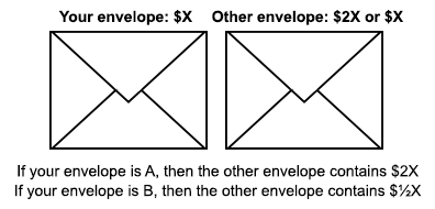
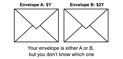
Newcomb’s problem: You find yourself in a room with two boxes in it. Box #1 is clear, and you can see $10,000 inside. Box #2 is opaque. A loud voice announces to you: “Box 2 has either 1 million dollars inside of it or nothing. You have a choice: Either you take just Box 2 by itself, or you take both Box 1 and Box 2.”

As you’re reaching forward to take both boxes, the voice declares: “Wait! There’s a catch.

Sometime before you entered the room, a Predictor with enormous computing power scanned you, made an incredibly detailed simulation of you, and used it to make a prediction about what decision you would make. The Predictor has done similar simulations many times in the past, and has never been wrong. If the Predictor predicted that you would take just Box 2, then it filled up the box with 1 million dollars. And if the Predictor predicted that you would take both boxes, then it left Box 2 empty. Now you may make your choice.”

Newcomb.png

The most initially intuitive answer to most people is to take both boxes. Here’s the strongest argument for why this makes sense, presented by Claus the causal thinker.

Claus: “The Predictor has already made its prediction and fixed the contents of the box. So we know for sure that my decision can’t possibly have any impact on whether Box 2 is full or empty. And in either case, I am better off taking both boxes than just one! Think about it like this: whether I one-box or two-box, I still end up taking Box 2. So let’s consider Box 2 taken – I have no choice in the matter. Now the only real question is if I’m also going to take Box 1. And Box 1 has $10,000 inside it! I can see it right there! My choice is really whether to take the free $10,000 or not, and I’d be a fool to leave it behind.”

***

Claus makes a very convincing argument. On his calculation, the expected value of two-boxing is strictly greater than the expected value of one-boxing, regardless of what probabilities he puts on the second box being empty. We’ll call this the dominance argument.

But Claus is making a fundamental error in his calculation. Let’s let a different type of decision theorist named Eve interrogate Claus.

Eve: “So, Claus, I’m curious about how you arrived at your answer. You say that your decision about whether or not to take Box 1 can’t possibly impact the contents of Box 2. I think that I agree with this. But do you agree that if you don’t take Box 1, it is more likely that Box 2 has a million dollars inside it?”

Claus: “I can’t see how that could be the case. The box’s contents are already fixed. How could my decision about something entirely causally unrelated make it any more likely that the contents are one way or the other?”

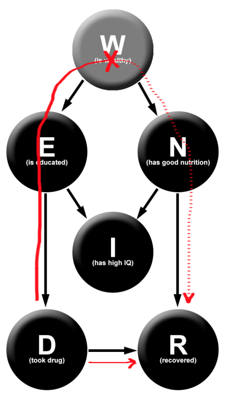
Eve: “Well, it’s not actually that unusual. There are plenty of things that are correlated without any direct causal impact between them. For example, say that a certain gene causes you to be a good juggler, but also causes a high chance of a certain disease. In this case, juggling ability and incidence of the disease will end up being correlated in the population, even though neither one is directly causing the other. And if you’re a good juggler, then you should be more worried that maybe you also have the disease!”

Claus: “Sure, but I don’t see how that case is anything like this one…”

Eve: “The two cases are actually structurally identical! Let me draw some causal diagrams…” (Claus rummages around for paper and a pencil)

Newcomb vs Juggling alt.png

Eve: “In our disease example, we have a common cause (the gene) that is directly causally linked to both the disease and to being a good juggler. So the “disease” variable and the “good juggler” variable are dependent because of the “gene” variable. In your Newcomb problem, the common cause is your past self at the moment that the Predictor scanned you. This common cause is directly linked to both your decision to one-box or two-box in the present, and to the contents of the box. Which means that in the exact same way that being a good juggler makes you more likely to have the disease, two-boxing makes you more likely to end up with an empty Box 2! The two cases are exactly analogous!”

Claus: “Hmm, that all seems correct. But even if my decision to take Box 1 isn’t independent of the contents of Box 2, this doesn’t necessarily mean that I shouldn’t still take both.”

Eve: “Right! But it does invalidate your dominance argument, which implicitly rested on the assumption that you could treat the contents of the box as if they were unaffected by your action. While your actions do not strictly speaking causally effect the contents of the box, they do change the likelihoods of the different possible contents! So there is a real sense in which your actions do statistically affect the contents of the box, even though they don’t causally affect them. Anyway, we can just calculate the actual expected values and see whether one-boxing or two-boxing comes out ahead.”

Eve writes out some expected utility calculations:

Newcomb vs Juggling 2

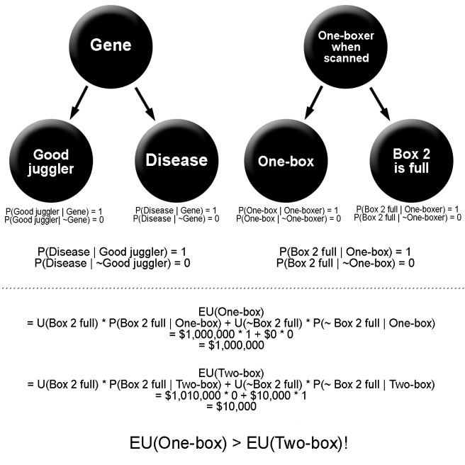
Eve: “So you see, it actually turns out to always be better to one-box than to two-box!”

Claus: “Hmm, I guess you’re right. Okay never mind, I guess that I’ll one-box. Thanks!”

***

Claus goes away for a while, and comes back a more sophisticated causal thinker.

Claus: “Hey, remember that I agreed that my decision and the contents of Box 1 are actually dependent upon each other, just not causally?”

Eve: “Yes.”

Claus: “Well, I do still agree with that. But I am also still a two-boxer. I’ll explain – would you hand me that paper?”

Claus scribbles a few equations beneath Eve’s diagrams.

EDT vs CDT.png

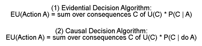
Claus: “When you calculated the expected values of one-boxing and two-boxing, you implicitly used Equation (1). Let’s call this equation the “Evidential Decision Algorithm.” You summed over all the possible consequences of your actions, and multiplied the values of each consequence by the conditional probability of that consequence, given the decision.”

Eve: “Yes…”

Claus: “Well, I have a different way to calculate expected values! It’s Equation (2), and I call it the “Causal Decision Algorithm.” I also sum over all possible consequences, but I multiply the value of each consequence by its causal conditional probability, not it’s ordinary conditional probability! And when you calculate the expected value, it turns out to be larger for two-boxing!”

Eve: “Hmm, doesn’t this seem a little arbitrary? Maybe a little ad-hoc?”

Claus: “Not at all! The point of rational decision-making is to choose the decision that causes the best outcomes. What we should be interested in is only the causal links between our decisions and their possible consequences, not the spurious correlations.”

Eve: “Hmm, I can see how that makes sense…”

Claus: “Here, let’s look back at your earlier example about juggling and disease. I agree with what you said that if you observe that you’re a good juggler, you should be worried that you have the disease. But imagine that instead of just observing whether or not you’re a good juggler, you get to decide whether or not to be a good juggler. Say that you can decide to spend many hours training your juggling, and at the end of that process you know that you’ll be a good juggler. Now, according to your decision theory, deciding to train to become a good juggler puts you at a higher risk for having the disease. But that’s ridiculous! We know for sure that your decision to become a good juggler does not make you any more likely to have the disease. Since you’re deciding what actions to take, you should treat your decisions like causal interventions, in which you set the decision variable to one value or another and in the process break all other causal arrows directed at it. And that’s why you should be using the causal conditional probability, not the ordinary conditional probability!”

Eve: “Huh. What you’re saying does have some intuitive appeal. But now I’m starting to think that there is an important difference that we both missed between the juggling example and Newcomb’s problem.”

Eve draws two more diagrams on a new page.

Newcomb vs Juggling 3.png

Eve: “In the juggling case, it makes sense to describe your decision to become a good juggler or not as a causal intervention, because this decision is not part of the chain of causes leading from your genes to your juggling ability – it’s a separate cause, independent of whether or not you have the gene. But in Newcomb’s problem, your decision to one-box or two-box exists along the path of the causal arrow from your past character to your current action! The Predictor predicted every part of you, including the part of you that’s thinking about what action you’re going to take. So while modeling your decision as a causal intervention in the juggling example makes sense, doing so in Newcomb’s case is just empirically wrong! Whatever part of your brain ends up deciding to “intervene” and two-box, the Predictor predicted that this would happen! By the nature of the problem, any way in which you attempt to intervene on your decision will inevitably not actually be a causal intervention.”

***

(Tim, a new type of decision theorist, appears in a puff of smoke)

Claus and Eve: “Gasp! Who are you?”

Tim: “I’m Tim, a new type of decision theorist! And I’m here to say that you’re both wrong!”

Claus and Eve: “Gasp!”

Tim: “I’ll explain with a thought experiment. You both know the prisoner’s dilemma, right? Two prisoners each get to make a choice either to cooperate or defect. The best outcome for each one is that they defect and the other prisoner cooperates, the second best outcome is that both cooperate, the second worst is that they both defect, and the worst is that they cooperate and the other prisoner defects. Famously, two rational agents in a prisoner’s dilemma will end up both defecting, because defecting dominates cooperating as a strategy. If the other prisoner defects, you’re better off defecting, and if the other prisoner cooperates, you’re better off defecting. So you should defect.”

Claus and Eve: “Yes, that seems right…”

Tim: “Well, first of all notice that two rational agents end up behaving in a sub-optimal way. They would both be better off if they each cooperated. But apparently, being ‘rational’ in this case entails ending up worse off. This should be a little unusual to you if you think that rational decision-making is about optimizing your outcomes. But now consider this variant: now you are in a prisoner’s dilemma with an exact clone of yourself. You have identical brains, have lived identical lives, and are now making this decision in identical settings. Now what do you do?”

Claus: “Well, on my decision theory, it’s still the case that I can’t causally effect my clone with my decision. This means that when I treat my decision as an intervention, I won’t end up making the probability that my clone defects given that I defect any higher. So defecting still dominates cooperating as a strategy. I defect!”

Eve: “Well, my answer depends on the set-up of the problem. If there’s some common cause that explains why my clone and I are identical (like maybe we were both manufactured in a twin-clone-making factory), then our decisions will be dependent. If I defect, then my clone will certainly defect, and if I cooperate, then my clone will cooperate. So my algorithm will tell me that cooperation maximizes expected utility.”

Tim: “There is no common cause. It’s by an insanely unlikely coincidence that you and your clone happen to have the same brains and to have lived the same lives. Until this moment, the two of you have been completely causally cut off from each other, with no possibility of any type of causal relationship .

Eve: “Okay, then I gotta agree with Claus. With no possible common cause and no causal intermediaries, my decision can’t affect my clone’s decision, causally or statistically. So I’ll defect too.”

Tim: “You’re both wrong. Both of you end up defecting, along with your clones, and everybody is worse off. Look, both of you ended up concluding that your decision and the decision of your clone cannot be correlated, because there are no causal connections to generate that correlation. But you and your clone are completely physically identical. Every atom in your brain is in a functionally identical spot as the atoms in your clone’s brain. Are you determinists?”

Eve: “Well, in quantum mechanics -”

Tim: “Forget quantum mechanics! For the purpose of this thought experiment, you exist in a completely deterministic world, where the same initial conditions lead to the same final conditions in every case, always. You and your clone are in identical initial conditions. So your final condition – that is, your decision about whether to cooperate or defect, must be the same. In the setup as I’ve described it, it is logically impossible that you defect and your clone cooperates, or that you cooperate and your clone defects.”

Claus: “Yes, I think you’re right… but then how do we represent this extra dependence in our diagrams? We can’t draw any causal links connecting the two, so how can we express the logical connection between our actions?”

Tim: “I don’t really care how you represent it in your diagram. Maybe draw a special fancy common cause node with special fancy causal arrows that can’t be broken towards both your decision and your clone’s decision.”

TDT Clones.png

Tim: “The point is: there are really only two possible worlds. In World 1, you defect and your clone defects. In World 2, you cooperate and your clone cooperates. Which world would you rather be in?”

Claus and Eve: “World 2.”

Tim: “Good! So you’ll both cooperate. Now, what if the clone is not exactly identical to you? Let’s say that your clone only ends up doing the same thing as you 99.999% of the time. Now what do you do?”

Claus: “Well, if it’s no longer logically impossible for my clone to behave differently from me, then maybe I should defect again?”

Tim: “Do you really want a decision theory that has a discontinuous jump in your behavior from a 99.999% chance to a 100% chance? I mean, I’ve told you that the chance that the clone gives a different answer than your answer is .001%! Rational agents should take into account all of their information, not only selective pieces of it. Either you ignore this information and end up worse off, or you take it into account and win!”

Eve: “Okay, yes, it seems reasonable to still expect a 99.999% chance of identical choices in this case. So we should cooperate again. But what does all of this have to do with Newcomb’s problem?”

Tim: “It relates to your answers to Newcomb’s problem in two ways. First, it shows that both of your decision algorithms are wrong! They are failing to take into account that extra logical dependency between actions and consequences that we drew with fancy arrows. And second, Newcomb’s problem is virtually identical to the prisoner’s dilemma with a clone!”

Eve and Claus: “Huh?”

Tim: “Here, let’s modify the prisoner’s dilemma in the following way: If you both cooperate, then you get one million dollars. If you cooperate and your clone defects, you get $0. If you defect and your clone cooperates, you get $1,010,000. And if you both defect, then you get $10,000. Now “cooperating” is the same as one-boxing, and “defecting” is the same as two-boxing!”

Eve: “But hold on, isn’t the logical dependency between my actions and my clone’s actions not carried over to the prisoner’s dilemma? Like, it’s not logically impossible that I one-box and the box has a million dollars in it, right?”

Tim: “It is with a perfect Predictor, yes! Remember, the Predictor works by creating a perfect simulation of you and seeing what it does. This means that your decision to one-box or to two-box is logically dependent on the Predictor’s prediction of what you do (and thus the contents of the box) in the exact same way that your decision to cooperate is logically dependent on your clone’s decision to one-box!”

TDT

Claus: “Yes, I see. So with a perfect Predictor, there are really only two worlds to consider: one in which I one-box and get a million dollars, and another in which I two-box and get just $10,000. And of course I prefer the first, so I should one-box.”

Tim: “Exactly! And if the Predictor is not perfectly accurate, and is only right 99.999% of the time…”

Eve: “Well, then there’s still only a .001% chance that I two-box and get an extra million bucks. So, I’m still much better off if I one-box than if I two-box.”

Tim: “Yep! It sounds like we’re all on the same page then. There’s a logical dependence between your action and the contents of the box that you are rationally required to take into account, and when you do take it into account, you end up seeing that one-boxing is the rational action.”

***

The decision theory that “Tim” is using is called timeless decision theory. It’s also been variously called functional decision theory, logical decision theory, and updateless decision theory.

Timeless decision theory ends up better off in Newcomb-like problems, invariably walking away with 1 million dollars instead of $10,000. It also does better than evidential decision theory (Eve’s theory) and causal decision theory (Claus’s theory) at prisoner’s-dilemmas-with-a-clone. These are fairly contrived problems, and it’d be easy for Eve or Claus to just deny that these problems have any real-world application.

But timeless decision theorists also cooperate with each other in ordinary prisoner’s dilemmas. They have a much easier time with coordination problems in general. They do better in bargaining problems. And they can’t be blackmailed in a large general class of situations. It’s harder to write these results off as strange quirks that don’t relate to real life.

A society of TDTs wouldn’t be plagued with doubts about the rationality of voting, wouldn’t find themselves stuck in as many sub-optimal Nash equilibria, and would look around and see a lot fewer civilizational inadequacies and low-hanging policy fruit than we currently have. This is what’s most interesting to me about TDT – that it gives a foundation for rational decision-making that seems like it has potential for solving real civilizational problems.