Sam Harris and the is-ought distinction

Sam Harris puzzles me sometimes.

I recently saw a great video explaining Hume’s is-ought distinction and its relation to the orthogonality thesis in artificial intelligence. Even if you are familiar with these two, the video is a nice and clear exposition of the basic points, and I recommend it highly.

Quick summary: Statements about what one ought to do are logically distinct from ‘is’ statements – those that simply describe the world. Statements in the second category cannot be derived from statements in the first, and vice versa. Artificial intelligence researchers recognize this in the form of the orthogonality thesis – an AI can have any combination of intelligence level and terminal values, and learning more about the world or becoming more intelligent will not result in value convergence.

This is more than just pure theory. When you’re building an AI, you actually have to design its goals separately from its capacity to describe and model the world. And if you don’t do so, then you’ll have failed at the alignment task – ensuring that the goals of the AI are friendly to humanity (and most of the space of all possible goals looks fairly unfriendy).

Said more succinctly: if you think that a sufficiently intelligent being that spends enough time observing the world and figuring out all of its “is” statements would naturally start to converge towards some set of “ought” statements, you’re wrong. While this may seem very intuitively compelling, it just isn’t the case. Values and beliefs are orthogonal, and if you think otherwise, you’d make a bad AI designer.

I am very confused by the existence of apparently reasonable people that have spent any significant amount of time thinking about this and have concluded that “ought”s can be derived from “is”s, or that “ought”s are really just some special type of “is”s.

Case in point: Sam Harris’s “argument” for getting an ought from an is.

Getting from “Is” to “Ought”

1/ Let’s assume that there are no ought’s or should’s in this universe. There is only what *is*—the totality of actual (and possible) facts.

2/ Among the myriad things that exist are conscious minds, susceptible to a vast range of actual (and possible) experiences.

3/ Unfortunately, many experiences suck. And they don’t just suck as a matter of cultural convention or personal bias—they really and truly suck. (If you doubt this, place your hand on a hot stove and report back.)

4/ Conscious minds are natural phenomena. Consequently, if we were to learn everything there is to know about physics, chemistry, biology, psychology, economics, etc., we would know everything there is to know about making our corner of the universe suck less.

5/ If we *should* to do anything in this life, we should avoid what really and truly sucks. (If you consider this question-begging, consult your stove, as above.)

6/ Of course, we can be confused or mistaken about experience. Something can suck for a while, only to reveal new experiences which don’t suck at all. On these occasions we say, “At first that sucked, but it was worth it!”

7/ We can also be selfish and shortsighted. Many solutions to our problems are zero-sum (my gain will be your loss). But *better* solutions aren’t. (By what measure of “better”? Fewer things suck.)

8/ So what is morality? What *ought* sentient beings like ourselves do? Understand how the world works (facts), so that we can avoid what sucks (values).

This is clearly a bad argument. Depending on what he intended it to be, step 5 is either a non sequitur or a restatement of his conclusion. It’s especially surprising because the mistake is so clearly visible.

I don’t know what to make of this, and really have no charitable interpretation. My least uncharitable interpretation is that maybe the root of the problem is an inability to let go of the longing to ground your moral convictions in objectivity. I’ve certainly had times where I felt so completely confident about a moral conviction that I convinced myself that it just had to be objectively true, although I always eventually came down from those highs.

I’m not sure, but this is something that I am very confused about and want to understand better.

Two envelopes paradox

In front of you are two envelopes, each containing some unknown amount of money. You know that one of the envelopes has twice the amount of money of the other, but you’re not sure which one that is and can only take one of the two. You choose one at random, and start to head out, when a thought goes through your head:

You: “Hmm, let me think about this. I just took an introductory decision theory class, and they said that you should always make decisions that maximize your expected utility. So let’s see… Either I have the envelope with less money or not. If I do, then I stand to double my money by switching. And if I don’t, then I only lose half my money. Since the possible gain outweighs the possible loss, and the two are equally likely, I should switch!”

Excited by your good sense in deciding to consult your decision theory knowledge, you run back and take the envelope on the table instead. But now, as you’re walking towards the door, another thought pops into your head:

You: “Wait a minute. I currently have some amount of money in my hands, and I still don’t know whether I got the envelope with more or less money. I haven’t gotten any new information in the past few moments, so the same argument should apply… if I call the amount in my envelope Y, then I gain $2Y by switching if I have the lesser envelope, and only lose $½Y by switching if I have the greater envelope. So… I should switch again, I guess!”

Slightly puzzled by your own apparently absurd behavior, but reassured by the memories of your decision theory professor’s impressive-sounding slogans about instrumental rationality and maximizing expected utility, you walk back to the table and grab the envelope you had initially chosen, and head for the door.

But a new argument pops into your head…

You see where this is going.

What’s going on here? It appears that by a simple application of decision theory, you are stuck switching envelopes ad infinitum, foolishly thinking that as you do so, your expected value is skyrocketing. Has decision theory gone crazy?

***

This is the wonderful two-envelopes paradox. It’s one of my favorite paradoxes of decision theory, because it starts from what appear to be incredibly minimal assumptions and produces obviously outlandish behavior.

If you’re not convinced yet that this is what standard decision theory tells you to do, let me formalize the argument and write out the exact calculations that lead to the decision to switch.

Call the envelope with less money “Envelope A”
Call the envelope with more money “Envelope B”
Call the envelope you are holding “Envelope E”
X = the amount of money in your envelope

First framing

P(E is A) = P(E is B) = ½
If E is A & you switch, then you get $2X
If E is B & you switch, then you get $½X
If E is A & you stay, then you get $X
If E is B & you stay, then you get $X

EU(switch) = P(E is A) · 2X + P(E is B) · ½X = 1¼ X
EU(stay) = P(E is A) · X + P(E is B) · X = X
So, EU(switch) > EU(stay)!

If you think that the conclusion is insane, then either there’s an error somewhere in this argument, or we’ve proven that decision theory is insane.

It’s easy to put forward additional arguments for why the expected utility should be the same for switching and staying, but this still leaves the nagging question of why this particular argument doesn’t work. The ultimate reason is wonderfully subtle and required several hours of agonizing for me to grasp.

I suggest you stop and analyze the argument a little bit before reading on – try to figure out for yourself what’s wrong.

Let me present the correct line of reasoning for comparison:

Call the envelope with less money “Envelope A”
Call the envelope with more money “Envelope B”
Call the envelope you are holding “Envelope E”
Label the amount of money in Envelope A = Y.
Then the amount of money in Envelope B = 2Y.

Second framing

P(E is A) = P(E is B) = ½
If E is A and you switch, then you get $2Y
If E is B and you switch, then you get $Y
If E is A and you stay, then you get $Y
If E is B and you stay, then you get $2Y

EU(switch) = P(E is A) · 2Y + P(E is B) · Y = 1½ Y
EU(stay) = P(E is A) · Y + P(E is B) · 2Y = 1½ Y
So EU(switch) = EU(stay)

This gives us the right answer, but the only apparent difference between this and what we did before is which quantity we give a name – X was the money in your envelope in the first argument, and Y is the money in the lesser envelope in this one. How could the answer depend on this apparently irrelevant difference?

***

Without further ado, let me diagnose the argument at the start of this post.

The fundamental mistake that this argument makes is that it treats the probability that you have the lesser envelope as if it is independent of the amount of money that you have in your hands. This is only the case if the amount of money in your envelope is irrelevant to whether you have the lesser envelope. But the amount of money in your hand is highly relevant information.

This may sound weird. After all, you chose the envelope at random, and shouldn’t the principle of maximum entropy prescribe that two equivalent envelopes are equally likely to be chosen? How could the unknown amount of money you’re holding have any sway over which one you were more likely to choose?

The answer is that the envelopes aren’t equivalent for any given amount of money in your hand. In general, given that you end up holding an envelope with $X, the chance that this is the lesser quantity is affected by the value of X.

Suppose, for example, that you know that the envelopes contain $1 and $2. Now in your mental model of the envelope in your hand, you see an equal chance of it containing $1 and $2. But now whether your envelope is the lesser or greater one is clearly not independent of the amount of money in your envelope. If you’re holding $1, then you know that you have the lesser envelope. And if you’re holding $2, then you know that you have the greater envelope.

In general, your prior probability over the possible amounts of money in your envelope will be relevant to the chance that you are holding the lesser or greater envelopes.

If you think that the envelopes are much more likely to contain small numbers, then given that the amount of money in your hand is large, you are much more likely to be holding the envelope with more money. Or if you think that the person stuffing the envelopes had only a certain fixed upper amount of cash that he was willing to put into the envelopes, then for some possible amounts of money in your envelope, you will know with certainty that it is the larger envelope.

Regardless, we’ll see that for any distribution of probabilities over the money in the envelopes, proper calculation of the expected utility will inevitably end up zero.

Here’s the sketch of the proof:

Stipulations:
Call the envelope with less money “Envelope A”
Call the envelope you are holding “Envelope E”
P(E is A) = P(E is B) = ½
If A has $x, then B has $2x
P(A has $x) = f(x) for some normalized function f(x)

The function f(x) represents your prior probability distribution over the possible amounts of money in A. We can infer your probability distribution over the possible amounts of money in B from the fact that B has double the money of A.

P(B has $x) = ½ P(A = $½ x) = ½ · f(½ x)

The ½ comes from the fact that we’ve stretched out our distribution by a factor of 2 and must renormalize it to keep our total probability equal to 1.

Now we’ll calculate the expected utility of switching, given that our envelope has some amount of money $x in it, and average over all possible values of x.

∆EU = < ∆EU given that E has $x >
= ∫ P(E has $x) · (∆EU given that E has $x) dx

Since this calculation will have several components, I’ll start color-coding them.

Next we’ll split up the calculation into the expected utility of switching (brown) and the expected utility of staying (blue).

∆EU = ∫ P(E has $x) · {EU(switch | E has $x) – EU(stay | E has $x)} dx

Our final subdivision of possible worlds will be regarding whether you’re holding the envelope with less or more money.

∆EU = ∫ P(E has $x) · { P(E is A | E has $x) · U(switch to B) + P(E is B | E has $x) · U(switch to A) – P(E is A | E has $x) · U(stay with A) + P(E is B | E has $x) · U(stay with B) } dx

We can rearrange the terms and color code them by whether they refer to the world in which you’re holding the lesser envelope (red) or the world in which you’re holding the greater envelope (green).

∆EU = ∫ { P(E has $x and E is A) · (U(switch to B)U(stay with A)) + P(E has $x and E is B) · (U(switch to A)U(stay with B)) } dx
= ∫ { P(A has $x) · P(E is A) · (2xx) + P(B has $x) · P(E is B) · (½ xx) } dx
= ∫ { f(x) · ½ x½ f(½ x) · ¼ x } dx
= ½ ∫ x f(x) dx – ½ ∫ (½ x) · f(½ x) · d(½ x)
= ½ ∫ x f(x) dx – ½ ∫ x’ f(x’) dx’

= 0

And we’re done!

So if this is the right way to do the calculation we attempted at the beginning, then where did we go wrong the first? The key is that we considered the unconditional probabilities P(E is A) and P(E is B) instead of the conditional probabilities P(E is A | E has $x) and P(E is B | E has $x).

This made the calculations more complicated, but was necessary. Why? Well, the assumption of independence of the value of your envelope and whether it is the lower or higher valued envelope is logically incoherent.

Proof in words: Suppose that your envelope’s value was independent of whether it is the lower or higher envelope. This means that for any value $X, it is equally likely that the other envelope contains $2X and that it contains $½X. We can write this condition as follows: P(other envelope has 2X) = P(other envelope has ½X) for all X. But there are no normalized distributions that satisfy this property! For any amount of probability mass in a given region [X, X+∆], there must also be at least as much probability mass in the region [4X, 4X+4∆]. Thus if any region has any finite probability mass, then that mass must be repeated an infinite number of times, meaning the distribution can’t be normalized! Proof by contradiction.

Even if we imagined some cap on the total value of a given envelope (say $1 million), we still don’t get away. Because now the value of your envelope is no longer independent of whether it is the lower or higher envelope! If the value of the envelope in your hands is $999,999, then you know for sure that you must have the larger of the two envelopes.

If the amount of money in your hands and the chance that you have the lesser envelope are independent, then you are imagining an unnormalizable prior. And if they are dependent, then the argument we started with must be amended to the colorful argument.

It’s not that at any point you get to look inside your envelope and see how much money is inside. It’s simply that you cannot talk about the probability of your envelope being the lesser of the two as if it is independent of the the amount of money you’re holding. And our starting argument did exactly that – it assumed that you were equally likely to have the smaller and larger envelope, regardless of how much money you held.

So the problem with our starting argument is wonderfully subtle. By the very framing of the statement “It’s equally likely that the other envelope contains $2X and $½X if my envelope contains $X,” we are committing ourselves to an impossibility: a prior probability with infinite total probability!

Principle of Maximum Entropy

Previously, I talked about the principle of maximum entropy as the basis of statistical mechanics, and gave some intuitive justifications for it. In this post I want to present a more rigorous justification.

Our goal is to find a function that uniquely quantifies the amount of uncertainty that there is in our model of reality. I’m going to use very minimal assumptions, and will point them out as I use them.

***

Here’s the setup. There are N boxes, and you know that a ball is in one of them. We’ll label the possible locations of the ball as:

B1, B2, B3, … BN
where Bn = “The ball is in box n”

The full state of our knowledge about which box the ball is in will be represented by a probability distribution.

(P1, P2, P3, … PN)
where Pn = the probability that the ball is in box n

Our ultimate goal is to uniquely prescribe an uncertainty measure S that will take in the distribution P and return a numerical value.

S(P1, P2, P3, … PN)

Our first assumption is that this function is continuous. When you make arbitrarily small changes to your distribution, you don’t get discontinuous jumps in your entropy. We’ll use this in a few minutes.

We’ll start with a simpler case than the general distribution – a uniform distribution, where the ball is equally likely to be in any of the N boxes.

For all n, Pn = 1/N

uniform-boxes.png

We’ll give the entropy of a uniform distribution a special name, labeled U for ‘uniform’:

S(1/N, 1/N, …, 1/N) = U(N)

Our next and final assumption is going to relate to the way that we combine our knowledge. In words, it will be that the uncertainty of a given distribution should be the same, regardless of how we represent the distribution. We’ll lay this out more formally in a moment.

Before that, imagine enclosing our boxes in M different containers, like this:

containers.png

Now we can represent the same state of knowledge as our original distribution by specifying first the probability that the ball is in a given container, and then the probability that it is in a given box, given that it is in that container.

Qn = probability that the ball is in container n
Pm|n = probability that the ball is in box m, given that it’s in container n

almost-final.png

Notice that the value of each Qn is just the number of boxes in the container divided by the total number of boxes. In addition, the conditional probability that the ball is in box m, given that it’s in container n, is just one over the number of boxes in the container. We’ll write these relationships as

Qn = |Cn| / N
Pm|n = 1 / |Cn|

The point of all this is that we can now formalize our third assumption. Our initial state of knowledge was given by a single distribution Pn. Now it is given by two distributions: Qn and Pm|n.

Since these represent the same amount of knowledge about which container the box is in, the entropy of each should be the same.

Final

And in general:

Initial entropy = S(1/N, 1/N, …, 1/N) = U(N)
Final entropy = S(Q1, Q2, …, QM) + ∑i Qi · S(P1|i, P2|i, …, PN|i)
= S(Q1, Q2, …, QM) + ∑i Qi · U(|Ci|)

The form of this final entropy is the substance of the uncertainty combination rule. First you compute the uncertainty of each individual distribution. Then you add them together, but weight each one by the probability that you encounter that uncertainty.

Why? Well, a conditional probability like Pm|n represents the probability that the ball is in box m, given that it’s in container n. You will only have to consider this probability if you discover that the ball is in container n, which happens with probability Qn.

With this, we’re almost finished.

First of all, notice that we have the following equality:

S(Q1, Q2, …, QM) = U(N) – ∑i [ Qi · U(|Ci|) ]

In other words, if we determine the general form of the function U, then we will have uniquely determined the entropy S for any arbitrary distribution!

And we can determine the general form of the function U by making a final simplification: assume that the containers all contain an equal number of boxes.

This means that Qn will be a uniform distribution over the M possible containers. And if there are M containers and N boxes, then this means that each container contains N/M boxes.

For all n, Qn = 1/M and |Cn| = N/M

If we plug this all in, we get that:

S(1/M, 1/M, …, 1/M) = U(N) – ∑i [1/M · U(N/M)]
U(M) = U(N) – U(N/M)
U(N/M) = U(N) – U(M)

There is only one continuous function that satisfies this equation, and it is the logarithm:

U(N) = K log(N) for some constant K

And we have uniquely determined the form of our entropy function, up to a constant factor K!

S(Q1, Q2, …, QM) = K log(N)  –  K ∑i Qi log(| Ci |)
= – K ∑i Qi log(| Ci |/N)
= – K ∑i Qi log(Qi)

If we add as a third assumption that U(N) should be monotonically increasing with N (that is, more boxes means more uncertainty, not less), then we can also specify that K should be a positive constant.

The three basic assumptions from which we can find the form of the entropy:

  1. S(P) is a continuous function of P.
  2. S should assign the same uncertainty to different representations of the same information.
  3. The entropy of a wide uniform distribution is greater than the entropy of a thin uniform distribution.

Consciousness

Every now and then I go through a phase in which I find myself puzzling about consciousness. I typically leave these phases feeling like my thoughts are slightly more organized on the problem than when I started thinking about it, but still feeling overwhelmingly confused about the subject.

I’m currently in one of those phases!

It started when I was watching an episode of the recent Planet Earth II series (which I recommend to everybody – it’s beautiful). One scene contains a montage of grizzly bears that have just emerged from hibernation and are now passionately grinding their backs against trees to shed their excess fur.

Nobody with a soul would watch this video and not relate to the back-scratching bears through memories of the rush of pleasure and utter satisfaction of a great back scratching session.

The natural question this raises is: how do we know that the bears are actually feeling the same pleasure that we feel when we get our backs scratched? How could we know that they are feeling anything at all?

A modest answer is that it’s just intuition. Some things just look to us like they’re conscious, and we feel a strong intuitive conviction that they really are feeling what we think they are.

But this is unsatisfying. ‘Intuition’ is only a good answer to a question when we have a good reason to presume that our intuitions should be reliable in the context of the question. And why should we believe that our intuitions about a rock being unconscious and a bear being conscious have any connection to reality? How can we rationally justify such beliefs?

The only starting point we have for assessing any questions about consciousness is our own conscious experience – the only one that we have direct and undeniable introspective access to. If we’re to build up a theory of consciousness, we must start there.

So for instance, we notice that there are tight correlations between patterns of neural activation in our brains and our conscious experiences. We also notice that there are some physical details that seem irrelevant to the conscious experiences that we have.

This distinction between ‘the physical details that are relevant to what conscious experiences I have’ and ‘the physical details that are irrelevant to what conscious experiences I have’ allow us to make new inferences about conscious experiences that are not directly accessible to us.

We can say, for instance, that a perfect physical clone of mine that is in a different location than me probably has a similar range of conscious experiences. This is because the only difference between us is our location, which is largely irrelevant to the range of my conscious experiences (I experience colors and emotions and sounds the same way whether I’m on one side of the room or another).

And we can draw similar conclusions about a clone of mine if we also change their hairstyle or their height or their eye color. Each of these changes should only affect our view of their consciousness insofar as we notice changes in our consciousness upon changes in our height, hairstyle, or eye color.

This gives us rational grounds on which to draw conclusions like ‘Other human beings are conscious, and likely have similar types of conscious experiences to me.’ The differences between other human beings and me are not the types of things that seem able to make them have wildly different types of conscious experiences.

Once we notice that we tend to reliably produce accurate reports about our conscious experiences when there are no incentives for us to lie, we can start drawing conclusions about the nature of consciousness from the self-reports of other beings like us.

(Which is of course how we first get to the knowledge about the link between brain structure and conscious experience, and the similarity in structure between my brain and yours. We probably don’t actually personally notice this unless we have access to a personal MRI, but we can reasonably infer from the scientific literature.)

From this we can build up a theory of consciousness. A theory of consciousness examines a physical system and reports back on things like whether or not this system is conscious and what types of conscious experiences it is having.

***

Let me now make a conceptual separation between two types of theories of consciousness: epiphenomenal theories and causally active theories.

Epiphenomenal theories of consciousness are structured as follows: There are causal relationships leading from the physical world to conscious experiences, and no causal relationships leading back.

Causally active theories of consciousness have both causal arrows leading from the physical world to consciousness, and back from consciousness to the physical world. So physical stuff causes conscious experiences, and conscious experiences have observable behavioral consequences.

Let’s tackle the first class of theories first. How could a good Bayesian update on these theories? Well, the theories make predictions about what is being experienced, but make no predictions about any other empirically observable behaviors. So the only source of evidence for these theories is our personal experiences. If Theory X tells me that when I hit my finger with a hammer, I will feel nothing but a sense of mild boredom, then I can verify that Theory X is wrong only through introspection of my own experiences.

But even this is unusual.

The mental process by which I verify that Theory X is wrong is occurring in my brain, and on any epiphenomenal theory, such a process cannot be influenced by any actual conscious experiences that I’m having.

If suddenly all of my experiences of blue and red were inverted, then any reaction of mine, especially one which accurately reported what had happened, would have to be a wild coincidence. After all, the change in my conscious experience can’t have had any causal effects on my behavior.

In other words, there is no reason to expect on an epiphenomenal theory of consciousness that the beliefs I form or the self-reports I produce about my own experiences should align with my actual conscious experiences.

And yet they invariably do. Every time I notice that I have accurately reported a conscious experience, I have noticed something that is wildly unlikely to occur under any epiphenomenal theory of consciousness. And by Bayes’ rule, each time this happens, all epiphenomenal theories are drastically downgraded in credence.

So this entire class of theories is straightforwardly empirically wrong, and will quickly be eliminated from our model of reality through some introspection. The theories that are left involve causation going both from the physical world to consciousness and back from consciousness to the physical world.

In other words, they involve two mappings – one from a physical system to consciousness, and another from consciousness to predicted future behavior of the physical system

But now we have a puzzle. The second mapping involves third-party observable physical effects that are caused by conscious experiences. But in our best understanding of the world, physical effects are always found to be the results of physical causes. For any behavior that my theory tells me is caused by a conscious experience, I can trace a chain of physical causes that uniquely determined this behavior.

What does this mean about the causal role of consciousness? How can it be true that conscious experiences are causal determinants of our behavior, and also that our behaviors are fully causally determined by physical causes?

The only way to make sense of this is by concluding that conscious experiences must be themselves purely physical causes. So if my best theory of consciousness tells me that experience E will cause behavior B, and my best theory of physics tells me that the cause of B is some set of physical events P, then E is equal to P, or some subset of P.

This is how we are naturally led to what’s called identity physicalism – the claim that conscious experiences are literally the same thing as some type of physical pattern or substance.

***

Let me move on to another weird aspect of consciousness. Imagine that I encounter an alien being that looks like an exact clone of myself, but made purely of silicon. What does our theory of consciousness say about this being?

It seems like this depends on if the theory makes reference only to the patterns exhibited by the physical structure, or to the physical structure itself. So if my theory is about the types of conscious experiences that arise from complicated patterns of carbon, then it will tell me that this alien being is not conscious. But if it just references the complicated patterns, and doesn’t specify the lower-level physical substrate from which the pattern arises, then the alien being is conscious.

The problem is that it’s not clear to me which of these we should prefer. Both make the same third-party predictions, and first-party verifications could only be made through a process involving a transformation of our body from one substrate to the other. In the absence of such a process, both of the theories make the exact same predictions about what the world looks like, and thus will be boosted or shrunk in credence exactly the same way by any evidence we receive.

Perhaps the best we could do is say that the first theory contains all of the complicated details of the first, but also has additional details, and so should be penalized by the conjunction rule? So “carbon + pattern” will always be less likely than “pattern” by some amount. But these differences in priors can’t give us that much, as they should in principle be dwarfed in the infinite-evidence limit.

What this amounts to is an apparently un-leap-able inferential gap regarding the conscious experiences of beings that are qualitatively different from us.

Inequality and free markets

(This post is a summary of the main things I found while diving into the economics literature on income inequality. Will try to condense my findings as much as possible, but there’s a lot to talk about. TL;DR at the end for lazy folk)

First, a note on terminology

Before getting into the published research on this topic, I started by surveying articles from popular news sources. I was curious to ultimately compare the standard media presentation to what I’d find in the scientific literature.

A large portion of what I read consisted of debates about the meanings of terms – one person says that capitalism is a lightly regulated market with a social safety net, another says any social safety net is socialism and therefore not capitalism, another says that a free market with any form of government regulation is corporatism, not capitalism, and they all yell at each other about terms and don’t get anything done.

By contrast, the terminology used in the economics and public policy literature was consistent, straightforward, and clear. I’ll define the controversial terms right here at the start to avoid confusion. These definitions are in line with the way that the terms are used in the literature.

Economic freedom: A combination of factors including limited regulation of businesses, protected rights to own private property, trade freedom, and small government.

Free marketAn economic system characterized by high degrees of economic freedom. Continue reading “Inequality and free markets”

40 papers on inequality in one sentence each

(Preliminary post – am planning to write this all up more digestibly in a future post)

***

Free markets and income inequality

Positive relationship

Capital in the 21st Century (Piketty)
When the rate of return on capital is greater than the rate of economic growth (as tends to occur in a free market given time), this leads to a concentration of wealth.

Capitalism and inequality: The negative consequences for humanity (Stevenson)
Inequalities are the inevitable result of capitalism, and we should abolish private property.

Envisioning Real Utopias (Wright)
Capitalism causes inequality through profit-seeking behavior and encouragement of innovation in technology.

How Privatization Increases Inequality (In the Public Interest)
Privatization of public goods causes inequality and inefficiency.

Income inequality and privatisation: a multilevel analysis comparing prefectural size of private sectors in Western China (Bakkeli)
More privatization corresponds to higher income inequality and lower individual outcome.

Economic Freedom, Income Inequality and Life Satisfaction in OECD Countries (Graafland, Lous)
Economic freedom causes higher income per capita, higher inequality, and overall lower happiness.

Negative relationship

Testing Piketty’s Hypothesis on the Drivers of Income Inequality: Evidence from Panel VARs with Heterogeneous Dynamics (Góes)
Piketty’s r – g hypothesis is wrong; the effect of r > g is not wealth concentration, but in fact mild wealth dispersion.

Economic Freedom and the Trade-off between Inequality and Growth (Scully)
Economic freedom overall reduces inequality, despite that economic growth increases inequality.

A Dynamic Analysis of Economic Freedom and Income Inequality in the 50 U.S. States: Empirical Evidence of a Parabolic Relationship (Bennett, Vedder)
Increases in economic freedom are associated with lower income inequality, and larger government is associated with greater inequality (with the exception of progressive taxation)

Economic freedom and equality: Friends or foes? (Berggren)
More economic freedom is associated with less inequality, because of trade liberalization and economic growth.

Economic Freedom And Income Inequality Revisited: Evidence From A Panel Error Correction Model (Apergis, Dincer, Payne)
Economic freedom reduces inequality in both the short and long run, and inequality causes less economic freedom.

Income inequality and economic freedom in the U.S. states (Ashby, Sobel)
More economic freedom causes larger per capita income, higher rates of economic growth, and less relative income inequality.

Other

On the ambiguous economic freedom–inequality relationship (Bennett, Nikolaev)
The relationship between economic freedom and inequality is ambiguous – it depends on how you choose your freedom and inequality measures.

***

Income inequality in the US

Trade

The Geography of Trade and Technology Shocks in the United States (Autor, Dorn, Hanson)
Two biggest causes of growing inequality are technology and trade, which are geographically separate in their effects.

Why are American Workers getting Poorer? China, Trade and Offshoring (Ebenstein, Harrison, McMillan)
Offshoring to China has led to US wage declines, but trade with China is much more important in explaining wage declines.

China Trade, Outsourcing and Jobs (Kimball, Scott)
China is a currency manipulator, encouraging a huge trade imbalance and hurting US workers.

The China Syndrome: Local Labor Market Effects of Import Competition in the United States (Autor, Dorn, Hanson)
China imports increase unemployment, lower labor force participation, and reduce wages in the US.

Technology

Rising Income Inequality: Technology, or Trade and Financial Globalization? (Jaumotte, Lall, Papageorgiou)
Technological progress is the primary cause of the rise of inequality in the last 2 decades, and increased globalization has had a minor impact.

World Economic Forum Outlook, April 2017: Gaining Momentum? (International Monetary Fund)
Decrease in bottom wages in advanced economies is driven mostly by technology and also by globalization.

It’s the Market: The Broad-Based Rise in the Return to Top Talent (Kaplan, Rauh)
Incomes at the top are driven by technological change in information and communications that increase the relative productivity of talented individuals through audience magnification.

Policy

Wage Inequality: A Story of Policy Choices (Mishel, Scmitt, Shierholz)
Income inequality is the result of erosion of the minimum wage value, decreased union power, industrial deregulation, traid policy, failure to use fiscal spending to stimulate the economy, bad monetary policy by the Fed, and rent-seeking behaviors from CEOs.

Controversies about the Rise of American Inequality: A Survey (Gordon, Dew-Becker)
Rising inequality is due to a low minimum wage, the decline in unionization, audience magnification, generous stock options, and unregulated corporate wage practices, not imports, immigration, or a lower labor share of income.

The Top 1 Percent in International and Historical Perspective (Alvaredo, Atkinson, Piketty, Saez)
Tax policy, decreased labor bargaining ability, and increased capital income explain the growing income share at the very top, not technology.

Rent-seeking

Declining Labor and Capital Shares (Barkai)
Capital shares have declined faster than labor shares in the last 30 years, and the decline of labor shares is due entirely to an increase in markups, which decreases output and consumer welfare.

The Pay of Corporate Executives and Financial Professionals as Evidence of Rents in Top 1 Percent Incomes (Bivens, Mishel)
CEO pay is driven by rent-seeking behavior.

Evidence for the Effects of Mergers on Market Power and Efficiency (Blonigen, Pierce)
Mergers in manufacturing from 1997 to 2007 haven’t significantly increased productivity or efficiency, but have increased markups.

Skill premium

Skills, education, and the rise of earnings inequality among the “other 99 percent” (Autor)
Income inequality is mostly due to an increasing skill premium, but is also due to a decline in the minimum wage value, automation, international trade, de-unionization, and regressive taxation.

Other

The long-run determinants of inequality: What can we learn from top income data? (Roine, Vlachos, Waldenström)
High growth benefits top income earners, tax progressiveness reduces top income shares, and trade openness doesn’t really do anything.

Why Hasn’t Democracy Slowed Rising Inequality? (Bonica, McCarty, Poole, Rosenthal)
Democracy hasn’t slowed the rise in inequality because of a political acceptance of free-market capitalism, immigration and a low turnout of poor voters, rising real income and wealth making social insurance less attractive, money influencing politics, and distortion of democracy through gerrymandering.

Billionaire Bonanza (Collins, Hoxie)
The people at the top are crazy rich and we should tax them.

***

More on free markets

Economic Freedom, Institutional Quality, and Cross-Country Differences in Income and Growth (Gwartney, Holcombe, Lawson)
More economic freedom leads to more rapid growth and higher income levels.

Economic Freedom of the World: 2017 Annual Report (Gwartney, Lawson, Hall)
Economic freedom is strongly correlated with rapid growth, higher average income per capita, lower poverty rates, higher income amount/share for the poorest 10%, higher life expectancy, more civil liberties and political rights, more gender equality, greater happiness, and better access to electricity, gas, and water supplies.

Agent-Based Simulations of Subjective Well-Being (Baggio, Papyrakis)
Economic growth weakly correlates with happiness, and pro-middle and balanced growth correspond to much higher levels of long-term happiness than pro-rich growth.

***

Decline of income inequality

Latin America

Deconstructing the Decline in Inequality in Latin America (Lustig, López-Calva, Ortiz-Juarez)
Income inequality declined in Latin American countries because of a declining skill premium and government redistribution.

China

Global Inequality Dynamics: New Findings from WID.world (Alvaredo, Chancel, Piketty, Saez, Zucman)
China’s top 1% income share has risen since 1980 (partially due to privatization), peaked near 2006, and is stable/slightly declining.

The great Chinese inequality turnaround (Kanbur, Wang, Zhang)
Drop in Chinese inequality is due to tightening of rural labor markets from migration, government investment in infrastructure in the rural sector, minimum wage policies, and social programs.

***

Views on inequality

The Challenge of Shared Prosperity (Rivkin, Mills, Porter)
Business leaders care about inequality, and it’s in their perceived self-interest to reduce inequality.

How Much (More) Should CEOs Make? A Universal Desire for More Equal Pay. (Kiatpongsan, Norton)
Everybody across all socioeconomic classes wants less inequality.

***

Minimum wage

Minimum Wages and Employment (Neumark, Wascher)
Most studies show that minimum wages reduce employment of low-wage workers.

The Effects of a Minimum-Wage Increase on Employment and Family Income (Congressional Budget Office)
Increases in minimum wage would cause unemployment but have a net positive real income effect.


Gregory Watson (and how to change the world)

When you feel like cynically proclaiming the impossibility of ever making any real progress, think about the story of Gregory Watson.

In 1982, Gregory Watson was a UT Austin undergrad struggling to think of a topic to write about for his political science paper.

He came across an old failed attempt to amend the Constitution, first proposed over 200 years earlier in 1789. The amendment prevented congressional pay raises from taking place until after an election, the idea being that a Congressman shouldn’t be able to just give themselves pay-raises willy-nilly, without first having to wait to be re-elected.

Gregory had a wild idea: maybe the amendment could still be passed. He looked into it, and found that amazingly, yes, the amendment process was still live. Deadlines for amendment ratification were introduced in 1917, over a hundred years before the amendment was proposed. So this amendment had never gotten a deadline.

Excited, he wrote up his paper on this, suggesting that this amendment could and should be sent out for ratification 200 years after its proposal. He turned in the paper to his teaching assistant, and… got a C.

Sure that there was a mistake, he appealed the grade to the professor, and… once more got a C.

His paper judged inadequate, Gregory began lobbying lawmakers, sending letters to members of Congress. Most responses were disappointingly negative – the amendment was 200 years old, and this sort of thing just wasn’t done. But he didn’t stop. He kept writing appeals to members of Congress for years, pushing them to bring this amendment to the floor of state legislatures.

Finally the tide shifted in the hail of Gregory’s determined appeals to state lawmakers.

Maine passed the amendment a year after his failed paper. Colorado approved the amendment 2 years later. Then five more states the next year. And 16 more states in the following four years.

By 1992, the 27th Amendment was ratified. And in 2017, his old professor signed a grade change form, changing Gregory’s grade to an A+.

An undergraduate political science student changed the United States’ Constitution, for the better. And was given a C for it.

The system can be exasperating, and cases like these are few and far between, but they do happen.


Statistical mechanics is wonderful

The law that entropy always increases, holds, I think, the supreme position among the laws of Nature. If someone points out to you that your pet theory of the universe is in disagreement with Maxwell’s equations — then so much the worse for Maxwell’s equations. If it is found to be contradicted by observation — well, these experimentalists do bungle things sometimes. But if your theory is found to be against the second law of thermodynamics I can give you no hope; there is nothing for it but to collapse in deepest humiliation.

 – Eddington

My favorite part of physics is statistical mechanics.

This wasn’t the case when it was first presented to me – it seemed fairly ugly and complicated compared to the elegant and deep formulations of classical mechanics and quantum mechanics. There were too many disconnected rules and special cases messily bundled together to match empirical results. Unlike the rest of physics, I failed to see the same sorts of deep principles motivating the equations we derived.

Since then I’ve realized that I was completely wrong. I’ve come to appreciate it as one of the deepest parts of physics I know, and mentally categorize it somewhere in the intersection of physics, math, and philosophy.

This post is an attempt to convey how statistical mechanics connects these fields, and to show concisely how some of the standard equations of statistical mechanics arise out of deep philosophical principles.

***

The fundamental goal of statistical mechanics is beautiful. It answers the question “How do we apply our knowledge of the universe on the tiniest scale to everyday life?”

In doing so, it bridges the divide between questions about the fundamental nature of reality (What is everything made of? What types of interactions link everything together?) and the types of questions that a ten-year old might ask (Why is the sky blue? Why is the table hard? What is air made of? Why are some things hot and others cold?).

Statistical mechanics peeks at the realm of quarks and gluons and electrons, and then uses insights from this realm to understand the workings of the world on a scale a factor of 1021 larger.

Wilfrid Sellars described philosophy as an attempt to reconcile the manifest image (the universe as it presents itself to us, as a world of people and objects and purposes and values), and the scientific image (the universe as revealed to us by scientific inquiry, empty of purpose, empty of meaning, and animated by simple exact mathematical laws that operate like clockwork). This is what I see as the fundamental goal of statistical mechanics.

What is incredible to me is how elegantly it manages to succeed at this. The universality and simplicity of the equations of statistical mechanics are astounding, given the type of problem we’re dealing with. Physicists would like to say that once they’ve figured out the fundamental equations of physics, then we understand the whole universe. Rutherford said that “all science is either physics or stamp collecting.” But you try to take some laws that tell you how two electrons interact, and then answer questions about how 1023 electrons will behave when all crushed together.

The miracle is that we can do this, and not only can we do it, but we can do it with beautiful, simple equations that are loaded with physical insight.

There’s an even deeper connection to philosophy. Statistical mechanics is about epistemology. (There’s a sense in which all of science is part of epistemology. I don’t mean this. I mean that I think of statistical mechanics as deeply tied to the philosophical foundations of epistemology.)

Statistical mechanics doesn’t just tell us what the world should look like on the scale of balloons and oceans and people. Some of the most fundamental concepts in statistical mechanics are ultimately about our state of knowledge about the world. It contains precise laws telling us what we can know about the universe, what we should believe, how we should deal with uncertainty, and how this uncertainty is structured in the physical laws.

While the rest of physics searches for perfect objectivity (taking the “view from nowhere”, in Nagel’s great phrase), statistical mechanics has one foot firmly planted in the subjective. It is an epistemological framework, a theory of physics, and a piece of beautiful mathematics all in one.

***

Enough gushing.

I want to express some of these deep concepts I’ve been referring to.

First of all, statistical mechanics is fundamentally about probability.

It accepts that trying to keep track of the positions and velocities of 1023 particles all interacting with each other is futile, regardless of how much you know about the equations guiding their motion.

And it offers a solution: Instead of trying to map out all of the particles, let’s course-grain our model of the universe and talk about the likelihood that a given particle is in a given position with a given velocity.

As soon as we do this, our theory is no longer just about the universe in itself, it is also about us, and our model of the universe. Equations in statistical mechanics are not only about external objective features of the world; they are also about properties of the map that we use to describe it.

This is fantastic and I think really under-appreciated. When we talk about the results of the theory, we must keep in mind that these results must be interpreted in this joint way. I’ve seen many misunderstandings arise from failures of exactly this kind, like when people think of entropy as a purely physical quantity and take the second law of thermodynamics to be solely a statement about the world.

But I’m getting ahead of myself.

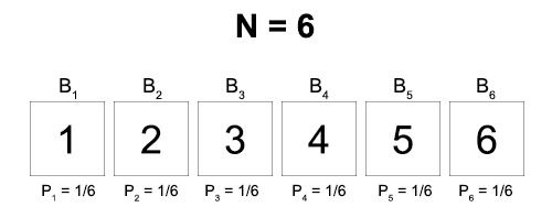
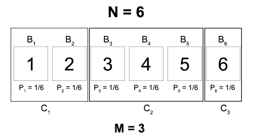
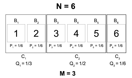
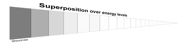
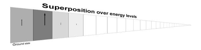
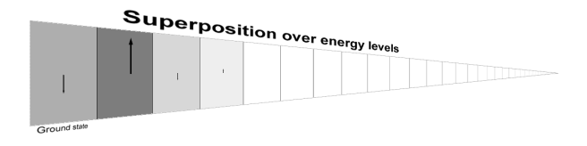
Statistical mechanics is about probability. So if we have a universe consisting of N = 1080 particles, then we will create a function P that assigns a probability to every possible position for each of these particles at a given moment:

P(x1, y1, z1, x2, y2, z2, …, xN, yN, zN)

P is a function of 3•1080 values… this looks super complicated. Where’s all this elegance and simplicity I’ve been gushing about? Just wait.

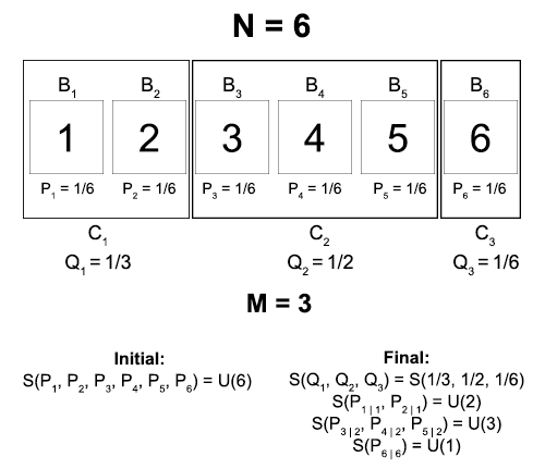
The second fundamental concept in statistical mechanics is entropy. I’m going to spend way too much time on this, because it’s really misunderstood and really important.

Entropy is fundamentally a measure of uncertainty. It takes in a model of reality and returns a numerical value. The larger this value, the more coarse-grained your model of reality is. And as this value approaches zero, your model approaches perfect certainty.

Notice: Entropy is not an objective feature of the physical world!! Entropy is a function of your model of reality. This is very very important.

So how exactly do we define the entropy function?

Say that a masked inquisitor tells you to close your eyes and hands you a string of twenty 0s and 1s. They then ask you what your uncertainty is about the exact value of the string.

If you don’t have any relevant background knowledge about this string, then you have no reason to suspect that any letter in the string is more likely to be a 0 than a 1 or vice versa. So perhaps your model places equal likelihood in every possible string. (This corresponds to a probability of ½ • ½ • … • ½ twenty times, or 1/220).

The entropy of this model is 20.

Now your inquisitor allows you to peek at only the first number in the string, and you see that it is a 1.

By the same reasoning, your model is now an equal distribution of likelihoods over all strings that start with 1.

The entropy of this model? 19.

If now the masked inquisitor tells you that he has added five new numbers at the end of your string, the entropy of your new model will be 24.

The idea is that if you are processing information right, then every time you get a single bit of information, your entropy should decrease by exactly 1. And every time you “lose” a bit of information, your entropy should increase by exactly 1.

In addition, when you have perfect knowledge, your entropy should be zero. This means that the entropy of your model can be thought of as the number of pieces of binary information you would have to receive to have perfect knowledge.

How do we formalize this?

Well, your initial model (back when there were 20 numbers and you had no information about any of them) gave each outcome a probability of P = 1/220. How do we get a 20 out of this? Simple!

Entropy = S = log2(1/P)

(Yes, entropy is denoted by S. Why? Don’t ask me, I didn’t invent the notation! But you’ll get used to it.)

We can check if this formula still works out right when we get new information. When we learned that the first number was a 1, half of our previous possibilities disappeared. Given that the others are all still equally likely, our new probabilities for each should double from 1/220 to 1/219.

And S = log2(1/(1/219)) = log2(219) = 19. Perfect!

What if you now open your eyes and see the full string? Well now your probability distribution is 0 over all strings except the one you see, which has probability 1.

So S = log2(1/1) = log2(1) = 0. Zero entropy corresponds to perfect information.

This is nice, but it’s a simple idealized case. What if we only get partial information? What if the masked stranger tells you that they chose the numbers by running a process that 80% of the time returns 0 and 20% of the time returns 1, and you’re fifty percent sure they’re lying?

In general, we want our entropy function to be able to handle models more sophisticated than just uniform distributions with equal probabilities for every event. Here’s how.

We can write out any arbitrary probability distribution over N binary events as follows:

(P1, P2, …, PN)

As we’ve seen, if they were all equal then we would just find the entropy according to previous equation: S = log2(1/P).

But if they’re not equal, then we can just find the weighted average! In other words:

S = mean(log2(1/P)) =∑ Pn log2(1/Pn)

We can put this into the standard form by noting that log(1/P) = -log(P).

And we have our general definition of entropy!

For discrete probabilities: S = – ∑ Plog Pn
For continuous probabilities: S = – ∫ P(x) log P(x) dx

(Aside: Physicists generally use a natural logarithm instead of log2 when they define entropy. This is just a difference in convention: e pops up more in physics and 2 in information theory. It’s a little weird, because now when entropy drops by 1 this means you’ve excluded 1/e of the options, instead of ½. But it makes equations much nicer.)

I’m going to spend a little more time talking about this, because it’s that important.

We’ve already seen that entropy is a measure of how much you know. When you have perfect and complete knowledge, your model has entropy zero. And the more uncertainty you have, the more entropy you have.

You can visualize entropy as a measure of the size of your probability distribution. Some examples you can calculate for yourself using the above equations:

Roughly, when you double the “size” of your probability distribution, you increase its entropy by 1.

But what does it mean to double the size of your probability distribution? It means that there are two times as many possibilities as you initially thought – which is equivalent to you losing one piece of binary information! This is exactly the connection between these two different ways of thinking about entropy.

Third: (I won’t name it yet so as to not ruin the surprise). This is so important that I should have put it earlier, but I couldn’t have because I needed to introduce entropy first.

So I’ve been sneakily slipping in an assumption throughout the last paragraphs. This is that when you don’t have any knowledge about the probability of a set of events, you should act as if all events are equally likely.

This might seem like a benign assumption, but it’s responsible for god-knows how many hours of heated academic debate. Here’s the problem: sure it seems intuitive to say that 0 and 1 are equally likely. But that itself is just one of many possibilities. Maybe 0 comes up 57% of the time, or maybe 34%. It’s not like you have any knowledge that tells you that 0 and 1 are objectively equally likely, so why should you favor that hypothesis?

Statistical mechanics answers this by just postulating a general principle: Look at the set of all possible probability distributions, calculate the entropy of each of them, and then choose the one with the largest entropy.

In cases where you have literally no information (like our earlier inquisitor-string example), this principle becomes the principle of indifference: spread your credences evenly among the possibilities. (Prove it yourself! It’s a fun proof.)

But as a matter of fact, this principle doesn’t only apply to cases where you have no information. If you have partial or incomplete information, you apply the exact same principle by looking at the set of probability distributions that are consistent with this information and maximizing entropy.

This principle of maximum entropy is the foundational assumption of statistical mechanics. And it is a purely epistemic assumption. It is a normative statement about how you should rationally divide up your credences in the absence of information.

Said another way, statistical mechanics prescribes an answer to the problem of the priors, the biggest problem haunting Bayesian epistemologists. If you want to treat your beliefs like probabilities and update them with evidence, you have to have started out with an initial level of belief before you had any evidence. And what should that prior probability be?

Statistical mechanics says: It should be the probability that maximizes your entropy. And statistical mechanics is one of the best-verified and most successful areas of science. Somehow this is not loudly shouted in the pages of every text on Bayesianism.

There’s much more to say about this, but I’ll set it aside for the moment.

***

So we have our setup for statistical mechanics.

  1. Coarse-grain your model of reality by constructing a probability distribution over all possible microstates of the world.
  2. Construct this probability distribution according to the principle of maximum entropy.

Okay! So going back to our world of N = 1080 particles jostling each other around, we now know how to construct our probability distribution P(x1, …, xN). (I’ve made the universe one-dimensional for no good reason except to pretty it up – everything I say follows exactly the same if I left it in 3D. I’ll also start writing the set of all N coordinates as X, again for prettiness.)

What probability distribution maximizes S = – ∫ P logP dX?

We can solve this with the method of Lagrange multipliers:

P [ P logP + λP ] = 0,
where λ is chosen to satisfy: ∫ P dX = 1

This is such a nice equation and you should do yourself a favor and learn it, because I’m not going to explain it (if I explained everything, this post would become a textbook!).

But it essentially maximizes the value of S, subject to the constraint that the total probability is 1. When we solve it we find:

P(x1, …, xN) = 1/VN, where V is the volume of the universe

Remember earlier when I said to just wait for the probability equation to get simple?

Okay, so this is simple, but it’s also not very useful. It tells us that every particle has an equal probability of being in any equally sized region of space. But we want to know more. Like, are the higher energy particles distributed differently than the lower energy?

The great thing about statistical mechanics is that if you want a better model, you can just feed in more information to your distribution.

So let’s say we want to find the probability distribution, given two pieces of information: (1) we know the energy of every possible configuration of particles, and (2) the average total energy of the universe is fixed.

That is, we have a function E(x1, …, xN) that tells us energies, and we know that the total energy E = ∫ P(x1, …, xN)•E(x1, …, xN) dX is fixed.

So how do we find our new P? Using the same method as before:

P [ P logP + λP + βEP ] = 0,
where λ is chosen to satisfy: ∫ P dX = 1
and β is chosen to satisfy: ∫ P•E dX = E

This might look intimidating, but it’s really not. I’ll write out how to solve this:

P [P logP + λP + βEP) ]
= logP + 1 + λ + βE = 0
So P = e-(1+λ) • e-βE
Renaming our first term, we get:
P(X) = 1/Z • e-βE(X)

This result is called the Boltzmann distribution, and it’s one of the incredibly important must-know equations of statistical mechanics. The amount of physics you can do with just this one equation is staggering. And we got it by just adding conservation of energy to the principle of maximum entropy.

Maybe you’re disturbed by the strange new symbols Z and β that have appeared in the equation. Don’t fear! Z is simply a normalization constant: it’s there to keep the probability of the total distribution at 1. We can calculate it explicitly:

Z = ∫ e-βE dX

And β is really interesting. Notice that β came into our equations because we had to satisfy this extra constraint about a fixed total energy. Is there some nice physical significance to this quantity?

Yes, very much so. β is what we humans like to call ‘temperature’, or more precisely, inverse temperature.

β = 1/T

While avoiding the math, I can just say the following: Temperature is defined to be the change in the energy of a system when you change its entropy a little bit. (This definition is much more general than the special case definition of temperature as average kinetic energy)

And it turns out that when you manipulate the above equations a little bit, you see that ∂SE = 1/β = T.

So we could rewrite our probability distribution as follows:

P(X) = 1/Z • e-E(X)/T

Feed in your fundamental laws of physics to the energy function, and you can see the distribution of particles across the universe!

Let’s just look at the basic properties of this equation. First of all, we can see that the larger E(X)/T becomes, the smaller the probability of a particle being in X becomes. This corresponds both to particles scattering away from high-energy regions and to less densely populated systems having lower temperatures.

And the smaller E(X)/T, the larger P(X). This corresponds to particles densely clustering in low-energy areas, and dense clusters of particles having high temperatures.

There are too many other things I could say about this equation and others, and this post is already way too long. I want to close with a final note about the nature of entropy.

I said earlier that entropy is entirely a function of your model of reality. The universe doesn’t have an entropy. You have a model of the universe, and that model has an entropy. Regardless of what physical reality is like, if I hand you a model, you can tell me its entropy.

But at the same time, models of reality are linked to the nature of the physical world. So for instance, a very simple and predictable universe lends itself to very precise and accurate models of reality, and thus to lower-entropy models. And a very complicated and chaotic universe lends itself to constant loss of information and low-accuracy models, and thus to higher entropy.

It is this second world that we live in. Due to the structure of the universe, information is constantly being lost to us at enormous rates. Systems that start out simple eventually spiral off into chaotic and unpredictable patterns, and order in the universe is only temporary.

It is in this sense that statements about entropy are statements about physical reality. And it is for this reason that entropy always increases.

In principle, an omnipotent and omniscient agent could track the positions of all particles at all times, and this agent’s model of the universe would be always perfectly accurate, with entropy zero. For this agent, the entropy of the universe would never rise.

And yet for us, as we look at the universe, we seem to constantly and only see entropy-increasing interactions.

This might seem counterintuitive or maybe even impossible to you. How could the entropy rise to one agent and stay constant for another?

Imagine an ice cube sitting out on a warm day. The ice cube is in a highly ordered and understandable state. We could sit down and write out a probability distribution, taking into account the crystalline structure of the water molecules and the shape of the cube, and have a fairly low-entropy and accurate description of the system.

But now the ice cube starts to melt. What happens? Well, our simple model starts to break down. We start losing track of where particles are going, and having trouble predicting what the growing puddle of water will look like. And by the end of the transition, when all that’s left is a wide spread-out wetness across the table, our best attempts to describe the system will inevitably remain higher-entropy than what we started with.

Our omniscient agent looks at the ice cube and sees all the particles exactly where they are. There is no mystery to him about what will happen next – he knows exactly how all the water molecules are interacting with one another, and can easily determine which will break their bonds first. What looked like an entropy-increasing process to us was an entropy-neutral process to him, because his model never lost any accuracy.

We saw the puddle as higher-entropy, because we started doing poorly at modeling it. And our models started performing poorly, because the system got too complex for our models.

In this sense, entropy is not just a physical quantity, it is an epistemic quantity. It is both a property of the world and a property of our model of the world. The statement that the entropy of the universe increases is really the statement that the universe becomes harder for our models to compute over time.

Which is a really substantive statement. To know that we live in the type of universe that constantly increases in entropy is to know a lot about the way that the universe operates.

More reading here if you’re interested!

Solution: How change arises in QM

Previously I pointed out that if you drew out the wave function of the entire universe by separating out its different energy components and shading each according to its amplitude, you would find that the universe appears completely static.

Energy superposition

This is correct according to standard quantum mechanics. If you looked at how much amplitude the universe had in any particular energy level, you would find that this amplitude was not changing in size.

The only change you would observe would be in the direction, or phase, of the amplitude in the complex plane. And directions of amplitudes in the complex plane are unphysical. Right?

No! While there is an important sense in which the direction of an amplitude is unphysical (the universe ultimately only computes magnitudes of amplitudes), there is a much much more important sense in which the direction of an amplitude contains loads of physical information.

This is because when the universe is in a superposition of different energy states, the amplitudes of these states can interfere.

It is here that we can find the answer to the question I posed in the previous post. Physical changes come from interference between the amplitudes of all the energy states that the universe is in superposition over.

One consequence of all of this is that if the universe did happen to be in a pure energy state, and not in a superposition of multiple energy levels, then change would be impossible.

From which we can conclude: The universe is in a superposition of energy levels, not in any clearly defined single energy level! (Proof: Look around and notice that stuff is happening)

This doesn’t mean, by the way, that the universe is actually in one of the energy levels and we just don’t know which. It also doesn’t mean that the universe is in some other distinct state found by averaging over all of the different energy states. “Superposition” is one of these funny words in quantum mechanics that doesn’t have an analogue in natural language. The best we can say is that the universe really truly is in all of the states in the superposition at once, and the degree to which it is in any particular state is the amplitude of that state.

***

Let’s imagine a simple toy universe with one dimension of space and one of time.

This universe is initially in an equal superposition of two pure energy states Φ0(x) and Φ1(x), each of which is a real function (no imaginary components). The first has zero energy, and we choose our units so that the second has an energy level equal to exactly 1.

So the wave function of our universe at time zero can be written Ψ = Φ0 + Φ1. (I’m ignoring normalization factors because they aren’t really crucial to the point here)

And from this we can conclude that our probability density is:

P(x) = Ψ*·Ψ = Φ02 + Φ12 + 2·Φ0·Φ1

Now we advance forward in time. Applying the Schrodinger equation, we find:

Φ0(x, t) = Φ0(x)
Φ1(x, t) = Φ1(x) · e-it

Notice that both of these energy states have a time-independent magnitude. The first one is obvious – it’s just completely static. The second one you can visualize as a function spinning in the complex plane, going from purely real and positive to purely imaginary to purely real and negative, et cetera. The magnitude of the function is just what you’d get by spinning it back to its positive real value.

From our two energy functions, we can find the total wave function of the universe:

Ψ(x, t) = Φ0(x) + Φ1(x) · e-it

Already we can see that our time-dependent wave function is not a simple product of our time-independent wave function and a phase.

We can see the consequences of this by calculating the time-dependent probability density:

P(x, t) = Φ0(x)2 + Φ1(x)2 + Φ0(x) · Φ1(x) · (e-it + eit)

Or…

P(x, t) = |Φ0|2 + |Φ1|2 + 2 · Φ0(x) · Φ1(x) · cos(t)

And in our final result, we can see a clear time dependence of the spatial probability distribution over the universe. The last term will grow and shrink, oscillating over time and giving rise to dynamics.

***

We can visualize what’s going on here by looking at the time evolution of each pure energy state as if it’s spinning in the complex plane. For instance, if the universe was in a superposition of the lowest four energy levels we would see something like:

4-Rotating.gif

The length of the arrow represents the amplitude of that energy level – “how much” the universe is in that energy state. The arrows are spinning in the complex plane with a speed proportional to the energy level they represent.

The wave function of the universe is represented by the sum of all of these arrows, as if you stacked each on the head of the previous. And this sum is changing!

For instance, in the universe’s first moment, the superposition looks like this:

4-Rotating T=0

And later the universe looks like this:

4-Rotating T=1

If we plotted out the first two energy states scaled by their amplitudes, we might see the following spatial distributions, initially and finally:

Even though there have been no changes in the magnitudes of the arrows (the degree to which the universe exists in each energy level) we get a very different looking universe.

This is the basic idea that explains all change in the universe, from the rising and falling of civilizations to the births and deaths of black holes: they are results of the complex patterns of interference produced by spinning amplitudes.

TIMN view of social evolution

(Papers here and here)

In the Neolithic era, societies are thought to have been mostly small groups bonded by kinship relations, with little social stratification. As technological advancement accommodated more complex social structures and larger groups of humans living together, problems of coordination became increasingly difficult. In response, more complex social structures arose, such as Chiefdoms, States and eventually Empires.

These structures solved coordination problems through a top-down command-and-control approach, enforced by strict hierarchical power structures. Historical exemplars of such structures include Ancient Egypt and the Roman Empire. These societies experienced immense growth, stretching out to dominate vast stretches of territory and millions of humans.

But as they grew, these societies began facing increasingly difficult problems of managing vast amounts of information involving complex exchanges and economic dynamics. Eventually, old mercantilist systems in which the state was in charge of economic transactions gave way to a grand new form of social structure: the market.

Societies that adopted market structures alongside the state became global leaders, dominating technological, social, and economic progress up until the present day. And just as previous forms of society had their distinctive failings, capitalistic societies face problems in the creation of social inequalities without the ability to address them.

Advances in technology that allow a revolutionary capacity for information exchange are resulting in the formation of a new form of social structure to address these problems. This structure is characterized by complicated heterarchical cooperation between massive networks of physically dispersed individuals, all coordinating on the basis of shared ideological aims. It is to them that the future belongs.

This is the view of history offered by political scientist David Ronfeldt, who framed the TIMN theory of social evolution.

If I were to summarize his entire theory in four sentences, I would say:

Societies through history can be explained through the interactions of four major forms of social structure: the Tribe, the Institution, the Market, and the Network. Each form defines a structure of governance and the way that individuals interact with one another, as well as cultural values and beliefs about the way society should be organized.

Each has different strengths and its weaknesses, and the progress of history has been a move towards adopting all four forms in a complicated balance. The future will belong to those societies that realize the potential of the network form and successfully incorporate it into their social structure.

There are a lot of parallels between this and previous things that I’ve read. I’ll go into that in a moment, but first will lay out more detailed definitions of his four primary structures.

The Tribe: Tribes are characterized by tight kinship relationships. Tribal social structures create strong senses of social identity and belonging, and define the culture of successive societies. They are small, egalitarian, and generally lack a strong leader. Their limitations are problems of administration and coordination as they grow, as well as nepotism and intertribal wars. Historical examples abound in the Neolithic era, and in modern times they exist in certain hot spots in Third World countries. In the First World, tribal patterns exist within families, urban gangs, civic clubs, and more abstractly in nationalism, racism and sports team mania.

The Institution: Institutions are characterized by authority figures, strict hierarchies, management structures, and administrative bureaucracies. Their strengths involve administration and solving coordination problems. They are afflicted with problems of corruption and abuse of power, as well as difficulty processing large amounts of information, leading to economic inefficiency. Examples include the great Empires, and they exist today in states, military organizations, religious organizations, and corporations.

The Market: Markets are characterized by competition and voluntary exchanges between self-interested individuals. They are uncentralized and nonhierarchical, and do well at handling enormous amounts of complex information and optimizing economic efficiency in exchanges of private goods. They lead to productive and innovative societies with thriving trade and commerce. Markets struggle to deal with externalities and lead to social inequality. Markets historically took off in the transition from mercantilism to capitalism in Europe, and are exemplified by the economies of the U.S. and the U.K. and more recently Chile, China, and Mexico.

The Network: Networks are characterized by cooperation between many autonomous individuals with no single central authority, where each individual is connected to all others. They are tied together not by blood or kinship relationships, but by ideology and common goals. Their strengths are yet to be seen, though Ronfeldt thinks that they could do well at promoting “group empowerment” and solving social issues. Same with their weaknesses, though he points vaguely in the direction of “information overload” and “deception”. Examples include social networks and transnational networks of NGOs.

Networks are the most poorly specified and speculative of the four forms. This is perhaps to be expected; after all, he thinks they have only begun to come into prominence at the advent of the Information Age.

They’re also the form that he stresses the most, making lots of breathless predictions about networked societies superseding the market-state societies that dominate the status quo. He urges states like the U.S. and the U.K. to become active participants in the ushering in of this great new era if they want to remain global leaders.

This part was less interesting to me. I’m not convinced that the problems of social inequality that he thinks Networks are necessary for cannot be fixed in a Market/State paradigm. All the same, it was nice to see falsifiable predictions from an otherwise highly theoretical work.

What I enjoyed most was his view of history. He sees the four forms as additive. When a society incorporates a new form, it does not discard the old, but builds upon it. Both end up modifying and influencing each other, and the end product is a combined system that incorporates both.

So for instance, the culture of a Tribe bleeds into its later instantiations as a State-run society, and can remain generations after the more visible tribal structures have passed on. And the adoption of free-market economic systems forces a reshaping of the State towards political democracy. He quotes Charles Lindblom:

However poorly the market is harnessed to democratic purposes, only within market-oriented systems does political democracy arise. Not all market-oriented systems are democratic, but every democratic system is also a market-oriented system. Apparently, for reasons not wholly understood, political democracy has been unable to exist except when coupled with the market. An extraordinary proposition, it has so far held without exception.

Ronfeldt explains this as a result of the market form pushing social values towards personal freedom, individuality, representation, and governmental accountability.

***

First connection:

I was reminded of psychologist Jonathan Haidt’s categorization of the different basic types of moral intuitions in The Righteous Mind. These are:

  • Care/Harm: Includes feelings like empathy and compassion. These intuitions are most triggered by experiences of vulnerable children, intense suffering and need, and cruelty.
  • Fairness/Cheating: Includes feelings of reciprocity, injustice, and equality. Triggered by others displaying cooperation or selfishness towards us.
  • Loyalty/Betrayal: Includes feelings of tribalism, unity and kinship. Triggered by involvement in tight groups
  • Authority/Subversion: Includes feelings of respect for parents, teachers, rulers, and religious leaders, as well as the feelings that this respect is owed. Involved in hierarchical thinking and perceptions of dominance relations.
  • Sanctity/Degradation: Includes feelings of disgust, purity, cleanliness, dirtiness, sacredness, and corruption.
  • Liberty/Oppression: Includes feelings of individualism, freedom, and resentment towards being dominated or oppressed.

Different political ideologies line up very well with different “moral foundations profiles”. Liberals tend to care primarily about the first two categories, Libertarians the last, and Conservatives a roughly equal mix of all six. You can take a questionnaire to see your personal moral profile here.

These categories look like they map really nicely onto the TIMN model as organizing principles for the different forms. Here’s my speculation on how the different social forms engage and capitalize on the different types of intuitions:

Tribes: Loyalty/Betrayal

Institutions: Authority/Subversion

Markets: Liberty/Oppression

Networks: Care/Harm?

The natural next question is what types of social forms would have as organizing principles the values of Fairness/Cheating or Sanctity/Degradation.

Second connection:

Sociologist Robert Nisbet attempted to categorize the different basic patterns of social interactions. He gave five categories: cooperation, conflict, exchange, coercion and conformity. For some reason this categorization seemed very deep to me when I first heard it, and it has stuck with me ever since.

Cooperation involves coordination between individuals that have a shared goal, while exchange involves coordination between individuals that are each motivated by their own self-interest.

Conflict occurs when individuals work against each other, competing for a larger share of rewards, for instance. Coercion is the forced cooperation between individuals with different goals. And conformity involves behavior that matches group expectations.

These categories nicely match the types of social interactions that characterize the different social forms in the TIMN model.

Tribes are a social form that are dominated by conformity interactions. Identity is tightly bound up with tribal culture, lineage, and adherence to social norms involving mutual defense and aid and who can have kids with whom.

The structure of Institutions is quite clearly analogous to coercion, and Markets to exchange and conflict. And by Ronfeldt’s description, Networks seem to be analogous to cooperative interactions.

Third connection:

Scott Alexander makes the point that democracies have several unique features that set them apart from previous forms of government.

These features all arise from the fact that democracies answer questions of leadership succession by handing them to the people. This is a big deal, for two main reasons:

First, democracies put an upper bound on how terrible a leader can be.

Why? The basic justification is that while the people don’t get to select the absolute best choice for leadership, they do get to select against the worst choices.

(FPTP is terrible enough that I actually don’t know if this is in general true. But this is in contrast to monarchical forms of government, which involve no feedback from the population, so the point stands.)

When the king of a hereditary monarchy dies and the throne passes to his oldest son, there is no formally recognized way to guard against the possibility that the kid is literally the next Hitler. At best, the population can just try to throw him out when they’ve had enough and let whoever wins out in the resulting scramble for power take over.

Second, democracy provides a great Schelling point for leadership succession.

(A Schelling point is a decision that would be arbitrary except that that is made on the basis of an expectation that everybody else will make the same decision. So if you’re supposed to meet a stranger in NYC, and you don’t know where, you’ll choose to go to Grand Central Terminal, and so will they. Not because of any psychic communication between the two of you, nor any sort of official designation of Grand Central Terminal as the One True Stranger Meeting Spot, but because you each expect the other to be there. Thus Grand Central Terminal is a geographical Schelling point for NYC.)

The Schelling point for leadership succession in a hereditary monarchy is royal blood. Which is to say that when the leader dies, everybody looks for the person (usually the man) with the most royal blood, and elects them.

But who determines if somebody’s blood is truly royal? What do you do if some other family decides that they have the truly royal blood? What if two people have equally royal blood?

The Schelling point for leadership succession in a theocratic monarchy like Ancient Egypt is the Official Word Of God.

Who determines which individual God actually wants in charge? What if two people both claim that God chose them to rule?

The problem is that these legitimacy claims are founded on fictions. There is no quality of royal-ness to blood, and there is no God to choose rulers.  In a democracy, the Schelling point for democracy is a real thing that is easily verifiable: the popular vote.

Everybody agrees who the correct leader is, because everybody can just look at the election results. And if somebody disagrees on who the correct leader is, then they have a clear action to take: mobilize voters to change their mind by the next election.

Thus democracy plays the dual role of ending succession squabbles and providing a natural pressure valve for those dissatisfied with the current leader.

These differences in structure seem really significant. I think that I would want to break apart Ronfeldt’s Institution category and replace it with two social forms: the Hierarchy and the Democracy.

A Hierarchy would be a social structure in which there is a strict top-down system of authority, and where the population at large does not have a formal role in determining who makes it at the top.

A Democracy also has a top-down system of power, but now also has a formal mechanism for feedback from the population to the top levels of power (e.g. an election). (I’d like a word for this that does not have as political a connotation, but failed to think of any)

***

The TIMN framework naturally leads to a story of the gradual progress of humans in our joint project of perfecting civilization. At each stage in history, new social structures arise to fix the failings of the old, and in this way forward-progress is made.

Overall, I think that the framework offers a potentially useful way of assessing different political and economic systems, by looking at the ways in which they utilize the strengths of these four structures and how they fall victim to the weaknesses.