Knots

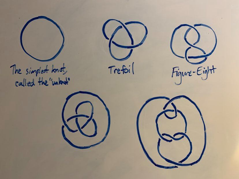
A knot is a closed loop in three dimensional space that doesn’t intersect itself. Some examples:

Knot diagrams are what you just saw: two dimensional representations of the three dimensional objects. It should be obvious that any one knot has many different diagrams. This raises an immediate question: given two knot diagrams, do they represent the same knot?

We need to be clear on what we mean by “the same knot”, of course. The intuition here is fairly obvious: you can rotate, stretch, and wiggle any section of a knot without fundamentally changing it.

What you CANNOT do is cut and reconnect the knot or pass one section of a knot through another of its sections.

Looking back at our starting five example knots, ask yourself if any of them represent the same knot:

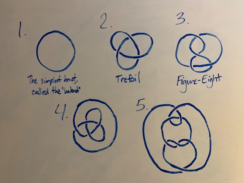
It might not be too obvious, but 2 and 4 represent the same knot, and so do 1 and 5! These equivalences (especially the equivalence between 1 and 5) should hopefully give a flavor for the difficulty of the general problem of determining equivalence between knots. While it’s sometimes possible to answer this by mere examination, it’s more often impossible. Even in cases where it seems very intuitively obvious (like, for instance, that the trefoil is not just an unknot in disguise), it’s hard to come up with a way to PROVE this fact.

When faced by a hard problem, we should begin thinking of the structure of a general solution. What we’d really like is a recipe for an algorithm that takes in two knot diagrams and decides whether they represent the same knots. (For economy of space and ease of reading, I’ll proceed to refer to “knot diagrams that represent equivalent knots” as “equivalent knot diagrams”.)

Here’s a naive first pass at a solution: Take either of the two knot diagrams you’re given. Start wiggling it around in all the allowed ways. At each step, check if you’ve obtained the other knot diagram. If you ever do, return True. Otherwise return False.

Maybe you see the problem here. In fact there are at least two major problems. (I said it was a naive first pass.)

The first big problem is in the “otherwise return False”. At what point in the algorithm do you actually reach this “otherwise” clause? Assuming that the two knot diagrams really do represent different knots, then you can keep manipulating the starting knot diagram in more and more complicated ways forever. At each stage you might get original knot diagrams, and at no stage are you justified in giving up and returning False. In other words, even if this algorithm worked as I described it, it could only ever decide equivalence of two equivalent knot diagrams. If handed two inequivalent knot diagrams, it would run forever. Thus this is really an algorithm for semi-deciding knot-diagram equivalence, not deciding it.

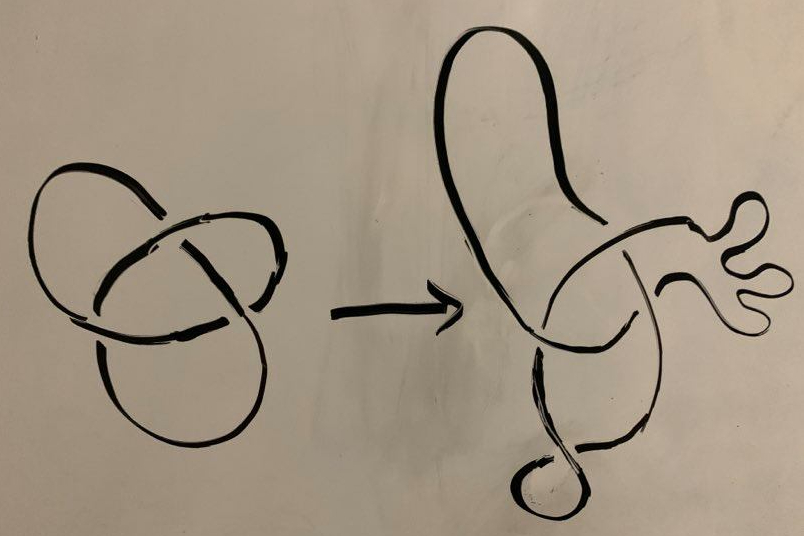
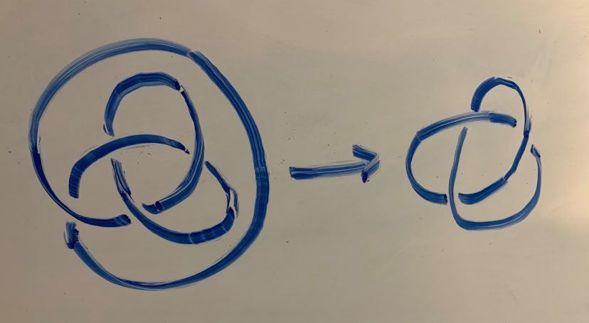
The second big problem is in the “start wiggling it around in all the allowed ways.” How would we describe the set of allowed transformations of a knot diagram to a computer? In particular, could we simplify down the allowed transformations to a finite set that would ensure that we really had done ALL possible manipulations? The answer to this is obviously no. Consider the following transformation:

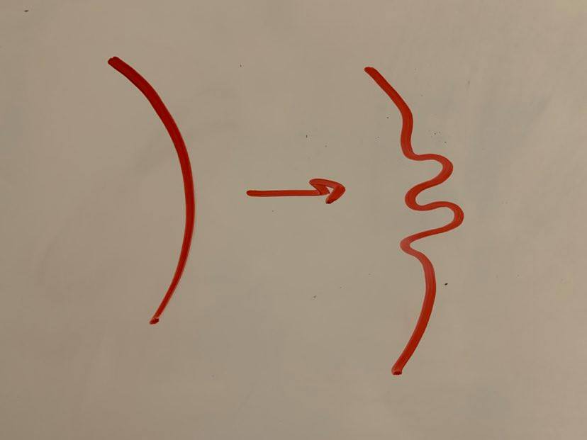
Each transformation like this produces a new knot diagram, simply by wiggling one side in an arbitrary way. But how many possible wiggles are there? Clearly an uncountable infinity: you can do arbitrarily small disruptions centered on any point along the knot, leaving the rest undisturbed, and get a distinct knot diagram each time.

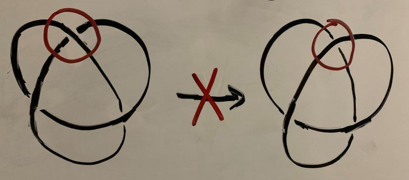
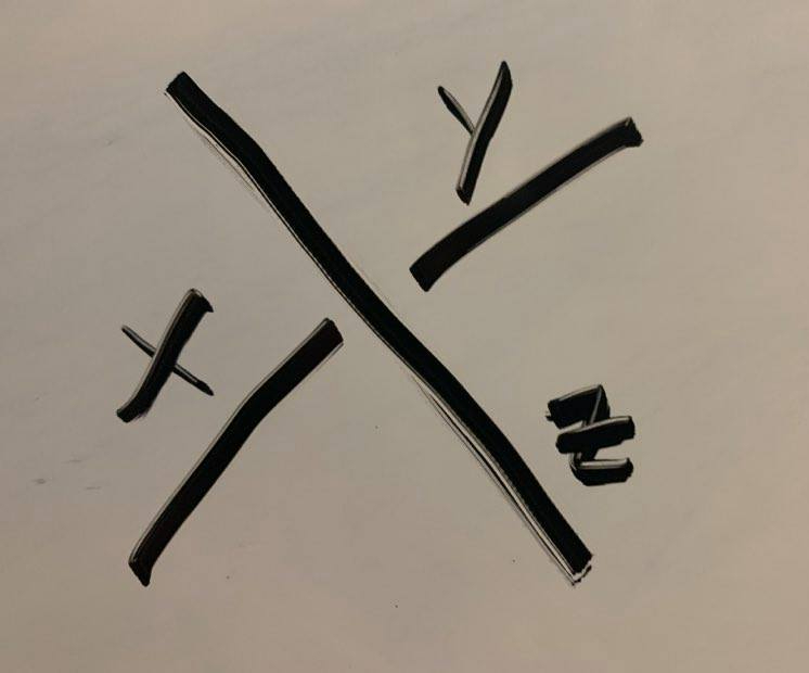
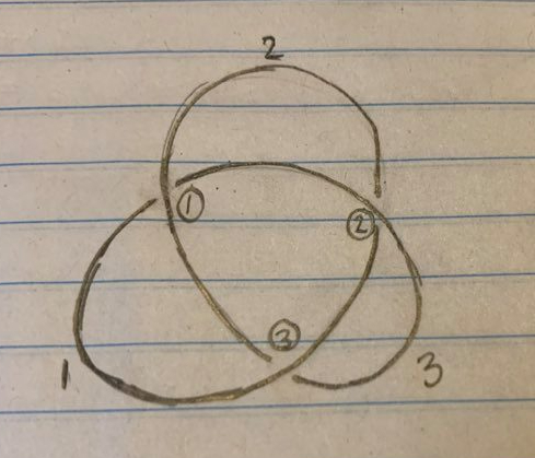
The “uncountable infinity” aspect of this second problem can actually be quickly resolved by sharpening our original question. Rather than regarding a knot diagram as any two-dimensional projection of a knot, we can think about a knot diagram as defined by its various crossings. For instance, we can label each uninterrupted “arc” in a knot diagram, as well as each crossing point.

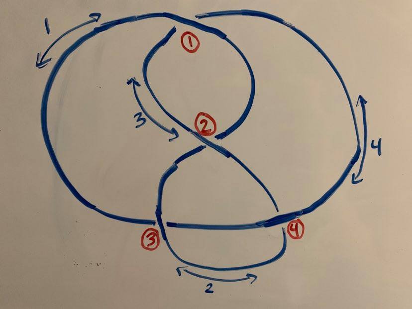
We now produce an alternative description of knot diagrams, obtained by describing how each arc interacts with each crossing point.

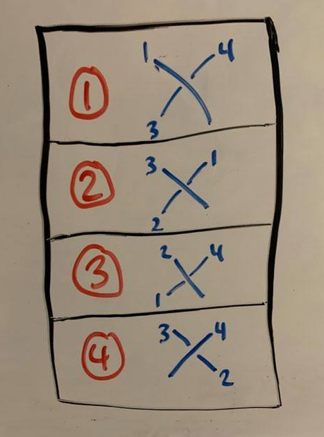
Crucially, our new description is not affected by the uncountably many small wiggles that do not make any substantial changes to the knot diagram. I.e., they do not affect the way that the various arcs cross under or above each other. We call this “equivalence of knot diagrams up to planar isotopy”, where planar isotopy is meant to refer to changes in a knot that don’t affect the structure of the crossings.

That’s one helpful step towards fixing up our algorithm. However, we are still in need of a finite set of transformations that we are sure generates ALL possible transformations on knot diagrams. I encourage you to think about this problem for a moment, and come up with a set of transformations to knot diagrams that you think are sufficient to produce knot diagrams.

(…)

(…)

I’ll leave a little space for you to try to come up with an answer for yourself. It’s not an easy exercise, but might be fun to test your knot-theoretic intuitions on.

(…)

(…)

Reidemeister Moves

It turns out that a set of six very simple transformations suffices for this task, discovered by Kurt Reidemeister. There are three categories of transformations:

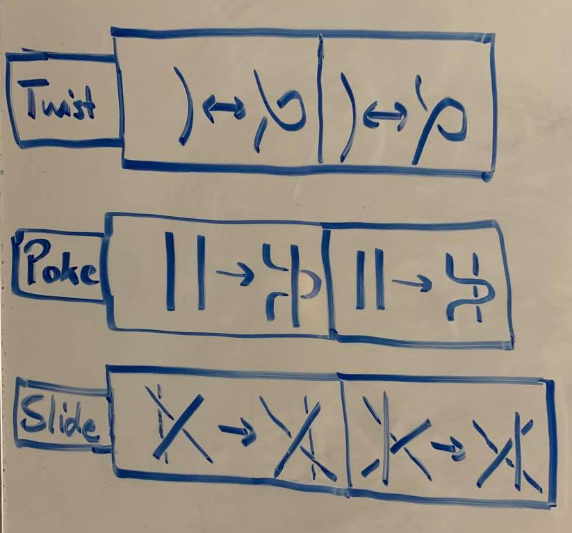
If two knot diagrams are equivalent, then there is a sequence of Reidemeister moves that transforms one to the other (up to planar isotopy).

It’s pretty fun to try to construct such sequences for oneself, and in doing so you’ll develop an intuition for why repeated Reidemeister moves suffice to generate all transformations. Try the earlier example of the two diagrams for the trefoil! I can do it in ten moves, can you do better?

So, this is great news! Our naive first attempt at building an algorithm to determine equivalence can be implemented (though it still only semi-decides equivalence rather than deciding it). Choose one of the diagrams, and run through all finite sequences of Reidemeister moves in any order. At each stage we check if we get the other diagram by application of these moves, and if so return True.

So with the help of the Reidemeister moves, we’ve successfully semidecided the equivalence problem. But it turns out that we can do better. Reidemeister moves not only allow us to determine that two diagrams are equivalent, but they lead us to a powerful tool to determine that two diagrams are inequivalent. The key concept here is invariants.

Invariants

Imagine that we found some quantity Q, calculated from a knot diagram, such that no matter how we alter the knot diagram, that quantity never changes. Now if we’re given two knot diagrams D₁ and D₂, and find that Q(D₁) ≠ Q(D₂), then we have conclusively demonstrated the inequivalence of the two diagrams! Why? Because if there was some way to transform D₁ into D₂, and since every transformation holds fixed Q(D₁), then Q(D₂) would have to equal Q(D₁)!

The hard part, of course, is finding invariants. But this is much easier when we have the help of Reidemeister moves! To show that Q(D) is an invariant quantity, all we need to do is show that the value of Q doesn’t change when we apply any Reidemeister move to the diagram D. This basically amounts to checking six simple cases, which is not too bad.

So, let’s go to our first invariant quantity: three-colorability.

3-Colorability

Three-colorability is quite simple: a knot is three-colorable if it’s possible to color each knot such that at each crossing either all three arcs are the same color, or all three are different.

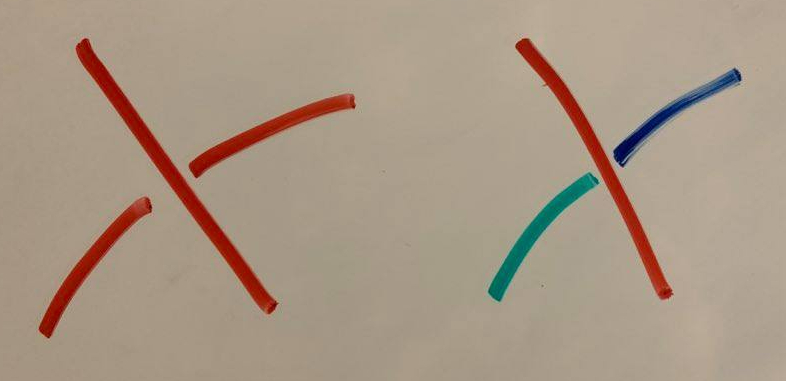
Notice that any knot can be trivially 3-colored by just letting every arc be the same color; to avoid this we add the requirement that for a 3-coloring to be valid, it must use at least two distinct colors.

It’s a fun exercise to show that this quantity is invariant using Reidemeister moves. The simplest case is the twist. Essentially all we need to do is show that if we apply a twist to a 3-colorable diagram, we can still 3-color the new diagram, AND that there’s a way to “untwist” a 3-colorable diagram so that we still retain 3-colorability. The proof is actually quite trivial; note that the crossing at any twist must be monochrome, since two of the involved arcs are actually the same.

Try convincing yourself that 3-colorabiity is preserved under the other Reidemeister moves!

So, 3-colorability is an invariant. There’s a very nice consequence of this. The trefoil is three-colorable, and the unknot (having only one arc) is not.

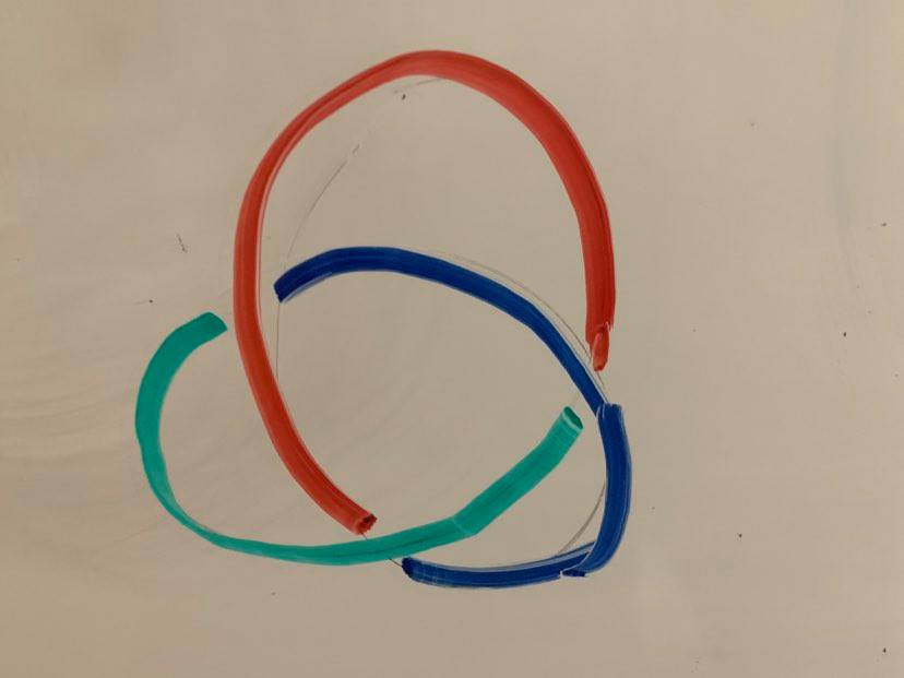
So this proves that the trefoil can not be unknotted! This was probably intuitively obvious from the outset, but we can now rest comfortably in the certainty of a mathematical proof.

p-Colorability

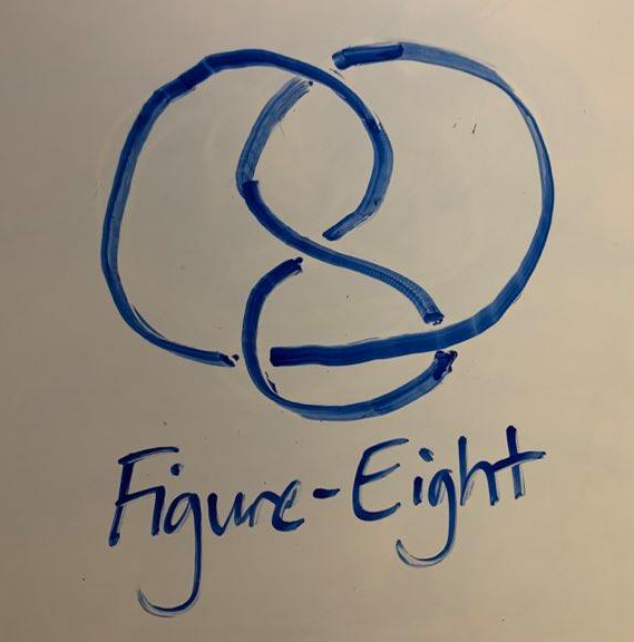
A fun exercise: try to 3-color the figure-eight knot, and see why it’s not possible.

This shows that the figure-eight knot is not equivalent to the trefoil. But what about the unknot? Neither the unknot and the figure-eight knot are 3-colorable, and yet they are not equivalent! So 3-colorability, while quite cool, isn’t the whole story. However, there’s a nice generalization of 3-colorability to p-colorability for any prime p.

Think about colors as numbers. So our set of three colors from the last section will just be {0, 1, 2}. A coloring is then a function mapping arcs to {0, 1, 2}. This gives us an algebraic way of expressing the 3-colorability property:

If x, y, and z are the colors of the three arcs connecting at a crossing, with z being the arc that passes above the crossing, then 2z – x – y = 0 (mod 3). It’s easily checkable that this is equivalent to the condition that each crossing is either monochrome, or else the three arcs are different colors.

We generalize this to any prime p as follows:

Our set of colors will be {0, 1, …, p – 1}. If for each crossing, 2z – x – y = 0 mod p, and at least two colors are used, then the knot is p-colorable.

For each prime p, p-colorability is an invariant, meaning that we have now gone from one invariant quantity to a countable infinity of invariants! We also can now distinguish the figure-eight knot from the unknot: the first is 5-colorable, while the unknot is not.

An exercise: try 5-coloring the trefoil. Is it possible?

However, this is not the end of the story. For one thing, it’s not so easy to determine if an arbitrary knot is p-colorable. It’s doable, sure, by trying all the possible colorings, but we want a quicker method. This will be addressed in the next section.

Much more importantly, we’ll see in the next section that there are knot diagrams that have the same colorability profile (i.e. D₁ is p-colorable iff D₂ is p-colorable, for each p), and yet represent different knots. So we need an even more powerful invariant to discriminate these from one another.

Knot Determinant

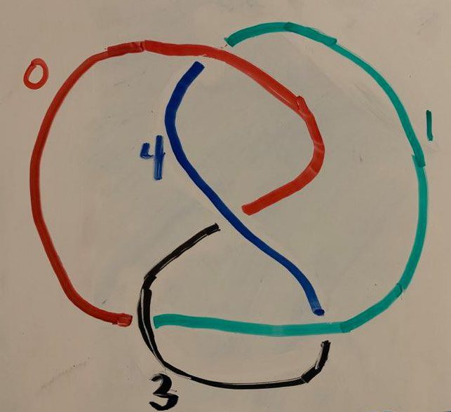
Take any knot and label its arcs and crossings with natural numbers.

Then construct a matrix M, where the (i, j) component corresponds to arc i and crossing j. If arc i isn’t involved in crossing j, then M_ij = 0. If arc i is involved in crossing j, and passes over it, then M_ij = 2. And if arc i passes under crossing j, then M_ij = -1.

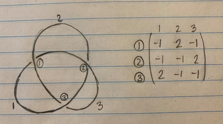
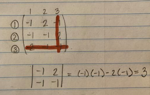
Now, cross out any row and column of your choice, and take the determinant of the remaining matrix. Take its absolute value, and you have the knot determinant.

You know what I’m going to say next: the knot determinant is an invariant! Not only is it an invariant, but it also fully determines the colorability profile of a knot! The rule is that if a knot has knot determinant N, then for any prime p > 2, N is p-colorable if and only if p divides N.

For instance, say we calculate that a knot has determinant 33. We immediately conclude that the knot is 3-colorable, 11-colorable, and not p-colorable for any other prime.

This is pretty incredible. We now have a simple deterministic procedure for looking at a knot diagram and producing a number that gives us the entire colorability profile of the knot. But wait, there’s more!

Suppose we have two knot diagrams, one with determinant 15, and the other with determinant 45. These two indicate the same colorability profile: 3-colorable, 5-colorable, and nothing else. But since the determinants are different, the two knots are not equivalent! In other words, any two knots with different determinants that have all the same prime factors (but with possibly different powers of those prime factors) will have the exact same colorability profile, and will nonetheless be proven inequivalent by the knot determinant!

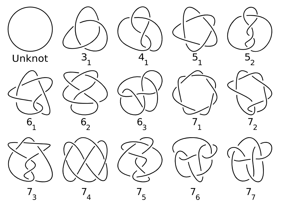
We’ve now reached the end of this dive into knot theory, but only because we’ve begun to near the end of my knowledge of the subject. By no means does the theory of knots end here. The knot determinant, amazing though it is, still does not fully pin down the different knots up to equivalence. There are distinct knots with the same determinant. If we were to dive further, we’d next look into a polynomial invariant, the Alexander polynomial. Going deeper, there’s hyperbolic invariants, involving the complement of a knot in hyperbolic space. Then there’s links, which are structures consisting of multiple knots linked together in some way, which have their own theory and periodic table. And we can even consider knotting spheres in four-dimensional space, or in general n-dimensional spheres in n+1-dimensional space! Plus there’s the operation of the knot sum, which we can use to combine distinct knots and get a new one. This operation is commutative and associative, and gives rise to the notion of prime and composite knots. And the coolness just keeps going on from here!

If nothing else, I hope I’ve convinced you that the subject of knots is of great mathematical interest and inspired you to look into it yourself. I’ll leave you with the first few rows of a (necessarily infinite) periodic table of knots, showing the prime knots up to seven crossings: