Consider the following simple model of the double-slit experiment:

A particle starts out at |O⟩, then evolves via the Schrödinger equation into an equal superposition of being at position |A⟩ (the top slit) and being at position |B⟩ (the bottom slit).

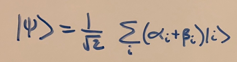
To figure out what happens next, we need to define what would happen for a particle leaving from each individual slit. In general, we can describe each possibility as a particular superposition over the screen.

Since quantum mechanics is linear, the particle that started at |O⟩ will evolve as follows:

If we now look at any given position |j⟩ on the screen, the probability of observing the particle at this position can be calculated using the Born rule:

Notice that the first term is what you’d expect to get for the probability of a particle leaving |A⟩ being observed at position |j⟩ and the second term is the probability of a particle from |B⟩ being observed at |j⟩. The final two terms are called interference terms, and they give us the non-classical wave-like behavior that’s typical of these double-slit setups.

Now, what we just imagined was a very idealized situation in which the only parts of the universe that are relevant to our calculation are the particle, the two slits and the detector. But in reality, as the particle is traveling to the detector, it’s likely going to be interacting with the environment. This interaction is probably going to be slightly different for a particle taking the path through |A⟩ than for a particle taking the path through |B⟩, and these differences end up being immensely important.

To capture the effects of the environment in our experimental setup, let’s add an “environment” term to all of our states. At time zero, when the particle is at the origin, we’ll say that the environment is in some state |ε₀⟩. Now, as the particle traverses the path to |A⟩ or to |B⟩, the environment might change slightly, so we need to give two new labels for the state of the environment in each case. |ε_A⟩ will be our description for the state of the environment that would result if the particle traversed the path from |O⟩ to |A⟩, and |ε_B⟩ will be the label for the state of the environment resulting from the particle traveling from |O⟩ to |B⟩. Now, to describe our system, we need to take the tensor product of the vector for our particle’s state and the vector for the environment’s state:

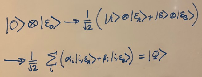
Now, what is the probability of the particle being observed at position j? Well, there are two possible worlds in which the particle is observed at position j; one in which the environment is in state |ε_A⟩ and the other in which it’s in state |ε_B⟩. So the probability will just be the sum of the probabilities for each of these possibilities.

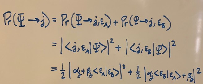
This final equation gives us the general answer to the double slit experiment, no matter what the changes to the environment are. Notice that all that is relevant about the environment is the overlap term ⟨ε_A|ε_B⟩, which we’ll give a special name to:

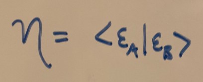
This term tells us how different the two possible end states for the environment look. If the overlap is zero, then the two environment states are completely orthogonal (corresponding to perfect decoherence of the initial superposition). If the overlap is one, then the environment states are identical.

And look what we get when we express the final probability in terms of this term!

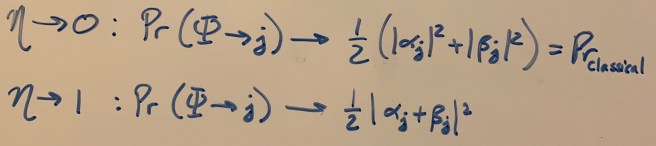
Perfect decoherence gives us classical probabilities, and perfect coherence gives us the ideal equation we found in the first part of the post! Anything in between allows the two states to interfere with each other to some limited degree, not behaving like totally separate branches of the wavefunction, nor like one single branch.